4  Project

XXXX

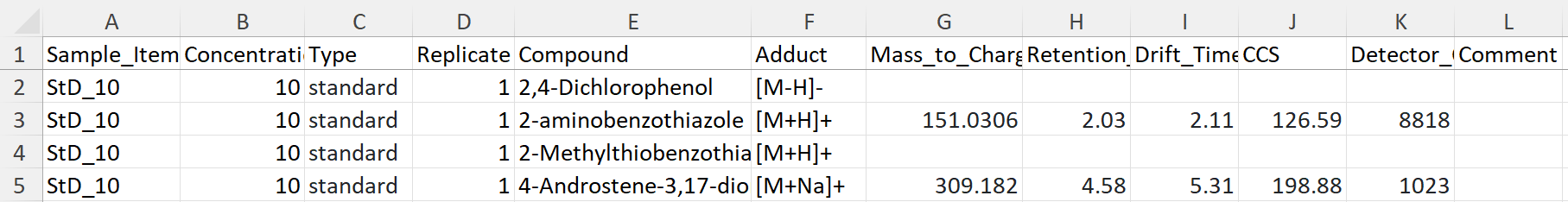
New format of Excel-sheet to work better to import in RStudio. It includes one column with the samples name, replicate number, target compound, which adduct it was detected as, the measured Mass_To_Charge ratio (m/z), Retention time (RT), Drift time (DT), CCS, and detector count (Intensity). All the data obtained from UNIFI software. The last column is for adding comments to a specific target compound.

Each type of sample has its own sheet. Hence, the data shown in the Figure 1, are from measurements of one standard called StD B, whereas measurements of another standard has another sheet in the same Excel-file. The first sheet in the file is called Info and contains information of the samples. For example, StD B is measured in different concentrations (10, 50, 100, 300, and 500 ppb). In the data for StD B, the Sample Items are called StD_XX, where XX is the concentration. However, in Info, it is possible to find the name of the measurements (e.g. StD_10_240319), number of replicates, and which standard and concentration that was measured.

Figure 1. Example of the format of the Excel sheet for imported data.

4.1 Loading of libraries

#Libraries
library(tidyverse)
library(readxl)
library(ggrepel)
library(ggpubr)
library(gt)
library(gtExtras)
library(viridis)
library(ggsci )
library(broom)
library(patchwork)

4.2 Functions

• \(MassError[ppm]=\frac{\textit{m/z}_{theretical}-\mathit{m/z}_{measured}}{\mathit{m/z}_{theoretical}}*10^6\)

#Function to calculate the Mass Error with three digits
mass_error <- function(mz_theoretical,mz_meaured){
  mass_error <- round((mz_theoretical-mz_meaured)/mz_theoretical*10^6, digits=3)
  return(mass_error)
}

• \(SEM=\frac{SD}{\sqrt{N}}\) , SD= Standard Deviation, N=number of samples

#Function to calculate the Standard Error of the Mean (SEM)
stderror <- function(x){
  round(sd(x, na.rm =TRUE)/sqrt(length(x)),4)
}

• Function for a Bar plot

#Uses quosure for the funciton
#bar_plot <- function(dataframe, xvalue, yvalue, fillvalue, error) {
#  xvalue <- enquo(xvalue)   # Capture xvalue as a quosure
#  yvalue <- enquo(yvalue)   # Capture yvalue as a quosure
#  fillvalue <- enquo(fillvalue)   # Capture fillvalue as a quosure
#  error <- enquo(error)   # Capture error as a quosure
  
#  p <- ggplot(data=dataframe, aes_string(x=quo_name(xvalue), y=quo_name(yvalue), fill=quo_name(fillvalue)))+
#    geom_bar(stat = "identity",position=position_dodge(0.9))+
#    geom_errorbar(aes(ymin=!!yvalue -!!error, 
#                      ymax=!!yvalue +!!error), 
#                  width=0.3, colour="black", size=0.8,position=position_dodge(0.9))+
#    scale_fill_npg()+
#    theme_minimal()+
#    theme(
#      panel.background = element_rect(fill = "white"),  # Set white background
#      panel.grid.major = element_blank(),  # Remove grid lines
#      panel.grid.minor = element_blank(),  # Remove grid lines
#      axis.text = element_text(size = 9),  # Increase font size of axis text
#      axis.title.y = element_text(size = 9,face = "bold"),  # Make y-axis label bold and italic
#      axis.text.y = element_text(color = "black", size = 9),  # Make x-axis text bold
#      axis.title.x = element_text(size = 10,face = "bold"),
#      axis.text.x = element_text(color = "black", size = 9, angle = 45, hjust=1),  # Make x-axis text bold
#      axis.ticks.x = element_line(color = "black"),  # Add ticks to x-axis in black color
#      axis.ticks.y = element_line(color = "black"),  # Add ticks to y-axis in black color
#      plot.margin = margin(0.5, 0.5, 0.4, 0.5, "cm"),  # Set plot margins
#      legend.text=element_text(size=9),
#      legend.background = element_rect(fill="white",
#                                     size=0.5, linetype="solid", 
#                                     colour ="black"),
#      legend.title = element_blank(),
#  )
#return(p)
#}

#uses embrace-operator ({{ }}) from Tidyverse insetad of quosure
bar_plot <- function(dataframe, xvalue, yvalue, fillvalue, error) {

  p <- ggplot(data=dataframe, aes(x={{ xvalue }}, y={{ yvalue }}, fill={{ fillvalue }}))+
    geom_bar(stat = "identity",position=position_dodge(0.9))+
    geom_errorbar(aes(ymin={{ yvalue}} -{{error }}, 
                      ymax={{ yvalue }} +{{ error }}), 
                  width=0.3, colour="black", size=0.8,position=position_dodge(0.9))+
    scale_fill_npg()+
    theme_minimal()+
    theme(
      panel.background = element_rect(fill = "white"),  # Set white background
      panel.grid.major = element_blank(),  # Remove grid lines
      panel.grid.minor = element_blank(),  # Remove grid lines
      axis.text = element_text(size = 9),  # Increase font size of axis text
      axis.title.y = element_text(size = 9,face = "bold"),  # Make y-axis label bold and italic
      axis.text.y = element_text(color = "black", size = 9),  # Make x-axis text bold
      axis.title.x = element_text(size = 10,face = "bold"),
      axis.text.x = element_text(color = "black", size = 9, angle = 45, hjust=1),  # Make x-axis text bold
      axis.ticks.x = element_line(color = "black"),  # Add ticks to x-axis in black color
      axis.ticks.y = element_line(color = "black"),  # Add ticks to y-axis in black color
      plot.margin = margin(0.5, 0.5, 0.4, 0.5, "cm"),  # Set plot margins
      legend.text=element_text(size=9),
      legend.background = element_rect(fill="white",
                                     size=0.5, linetype="solid", 
                                     colour ="black"),
      legend.title = element_blank(),
  )
return(p)
}

• Function for a Scatter plot

#uses embrace-operator ({{ }}) from Tidyverse insetad of quosure
scatter_plot <- function(dataframe, xvalue, yvalue, colorvalue, error) {
  #xvalue <- enquo(xvalue)   # Capture xvalue as a quosure
  #yvalue <- enquo(yvalue)   # Capture yvalue as a quosure
  #colorvalue <- enquo(colorvalue)   # Capture colorvalue as a quosure
  #error <- enquo(error)   # Capture error as a quosure
  
  p <- ggplot(data=dataframe, aes(x={{xvalue}}, y={{yvalue}}, color={{colorvalue}}))+
    geom_point()+
    geom_errorbar(aes(ymin = {{yvalue}} - {{error}}, 
                      ymax = {{yvalue}} + {{error}}),
                  width=0.7, colour="black", size=0.7) +
    
    scale_color_viridis(discrete=TRUE)+
    theme_minimal()+
    theme(
      panel.background = element_rect(fill = "white"),  # Set white background
      panel.grid.major = element_blank(),  # Remove grid lines
      panel.grid.minor = element_blank(),  # Remove grid lines
      axis.text = element_text(size = 9),  # Increase font size of axis text
      axis.title.y = element_text(size = 9,face = "bold"),  # Make y-axis label bold and italic
      axis.text.y = element_text(color = "black", size = 9),  # Make x-axis text bold
      axis.title.x = element_text(size = 10,face = "bold"),
      axis.text.x = element_text(color = "black", size = 9, angle = 45, hjust=1),  # Make x-axis text bold
      axis.ticks.x = element_line(color = "black"),  # Add ticks to x-axis in black color
      axis.ticks.y = element_line(color = "black"),  # Add ticks to y-axis in black color
      plot.margin = margin(0.5, 0.5, 0.4, 0.5, "cm"),  # Set plot margins
      legend.text=element_text(size=9),
      legend.background = element_rect(fill="white",
                                     size=0.5, linetype="solid", 
                                     colour ="black"),
      legend.title = element_blank(),
    )
####### TRIED TO MAKE ERROR AN OPTIONAL, SO IT ONLY PLOTS ERRORBARS IF ERROR IS NOT NULL ##########
  #if(!is.null(error)) {
    #error <- enquo(error)   # Capture error as a quosure
    #p <- p + geom_errorbar(aes(ymin = !!yvalue - !!error, 
    #                           ymax = !!yvalue + !!error),
    #                       width=0.7, colour="black", size=0.7)
    #}
####### DOES NOT WORK #############################
  return(p)
}

• Calculate concentration from calibration curve: \(Concentration =\frac{Response-Intercept}{Slope}\)

cal_conc <- function(response, intercept, slope){
  concentration <- (response-intercept)/slope
  return(concentration)
}

4.3 Target Compounds from UNIFI

This section is for data analysis when target compounds data (e.g. m/z, RT, DT, CCS, and intensity) has been obtained directly from UNIFI. Hence, the data has NOT been processed with e.g MS-DIAL, so there is not need to “find” the target compounds in a long list of features.

Importing the data

Two data sets are imported, one containing the measured data (data_hrms) and one with information of the target compounds (target_compounds), which contains the molecular formula, monoisotopic mass, and theoretical mass of the different adducts ([M+H]+, [M+Na]+, [M+NH4]+, and [M-H]-).

data_hrms <- read_excel("Data_HRMS_Format_TEST.xlsx", 
    sheet = "Data_StDB")
#glimpse(data_hrms)
target_compounds <- read_excel("Target_Compounds_StDB.xlsx")
#glimpse(target_compounds)

Calculate the Mass Accuracy with the mass_error() function depending on which adduct the compound was found as and add the results in the data_hrms data frame.

#If the compounds in target_compounds and data_hrms are in the same order
data_hrms <- data_hrms |> 
    mutate(Mass_accuracy=case_when(Adduct == "[M+H]+" ~ mass_error(target_compounds$`[M+H]+`, Mass_to_Charge_Ratio),
                              Adduct == "[M+Na]+" ~ mass_error(target_compounds$`[M+Na]+`, Mass_to_Charge_Ratio),
                              Adduct == "[M+NH4]+" ~ mass_error(target_compounds$`[M+NH4]+`, Mass_to_Charge_Ratio),
                             Adduct == "[M-H]-" ~ mass_error(target_compounds$`[M-H]-`,Mass_to_Charge_Ratio) )) 

#If the compounds in target_compounds and data_hrms are not in the same order, can join the two data frames according to the compounds name and then calculate mass accuracy
data_hrms <- inner_join(data_hrms, target_compounds, by = c("Compound" = "Item name")) |> 
    mutate(Mass_accuracy=case_when(Adduct == "[M+H]+" ~ mass_error(`[M+H]+`, Mass_to_Charge_Ratio),
                              Adduct == "[M+Na]+" ~ mass_error(`[M+Na]+`, Mass_to_Charge_Ratio),
                              Adduct == "[M+NH4]+" ~ mass_error(`[M+NH4]+`, Mass_to_Charge_Ratio),
                             Adduct == "[M-H]-" ~ mass_error(`[M-H]-`,Mass_to_Charge_Ratio) )) |> 
  select(Sample_Item, Replicate, Compound, Adduct, Mass_to_Charge_Ratio, Retention_Time, Drift_Time, CCS, Detector_Counts, Mass_accuracy)

Calculate the Average and SEM of m/z, Mass Accuracy, RT, DT, CCS, and intensity for each compound in each type of sample (Sample Item) with the mean() and SEM() functions.

data_hrms$Sample_Item <- factor(data_hrms$Sample_Item, levels=unique(data_hrms$Sample_Item)) #Convert Sample_Item to factor to be able to keep the original order of the data

data_hrms_average <-data_hrms |>  filter(!is.na(Mass_to_Charge_Ratio))|> 
  group_by(Sample_Item, Compound) |> 
  summarise(Average_MZ=round(mean(Mass_to_Charge_Ratio, na.rm =TRUE),digits=3),
            SEM_MZ=stderror(Mass_to_Charge_Ratio),
            Average_MassAccuracy=round(mean(Mass_accuracy, na.rm =TRUE),digits=3),
            SEM_MassAccuracy=stderror(Mass_accuracy),
            Average_RT=round(mean(Retention_Time, na.rm =TRUE),digits=3),
            SEM_RT=stderror(Retention_Time),
            Average_DT=round(mean(Drift_Time, na.rm =TRUE),digits=3),
            SEM_DT=stderror(Drift_Time),
            Average_CCS=round(mean(CCS, na.rm =TRUE),digits=3),
            SEM_CCS=stderror(CCS),
            Average_intensity=round(mean(Detector_Counts, na.rm =TRUE),digits=3),
            SEM_intensity=stderror(Detector_Counts)) |> 
  ungroup() |> 
  group_by(Compound)

`summarise()` has grouped output by 'Sample_Item'. You can override using the
`.groups` argument.

#glimpse(data_hrms_average)

Plots using the bar_plot function.

p1 <- bar_plot(data_hrms_average, Compound, Average_MZ, Sample_Item, SEM_MZ)+
  labs(y = "Average Mass-To-Charge Ratio", x="")+
  scale_y_continuous(expand = expansion(add=c(0,30)))

Warning: Using `size` aesthetic for lines was deprecated in ggplot2 3.4.0.
ℹ Please use `linewidth` instead.

Warning: The `size` argument of `element_rect()` is deprecated as of ggplot2 3.4.0.
ℹ Please use the `linewidth` argument instead.

p2 <- bar_plot(data_hrms_average, Compound, Average_RT, Sample_Item, SEM_RT)+
  labs(y = "Average Retention time [min]", x="")+
  scale_y_continuous(expand = expansion(add=c(0,1)))

#(p1 / p2) #need patchwork package for this

bar_plot(data_hrms_average, Compound, Average_DT, Sample_Item, SEM_DT)+
  labs(y = "Average Drift time [ms]", x="")+
  scale_y_continuous(expand = expansion(add=c(0,0.11)))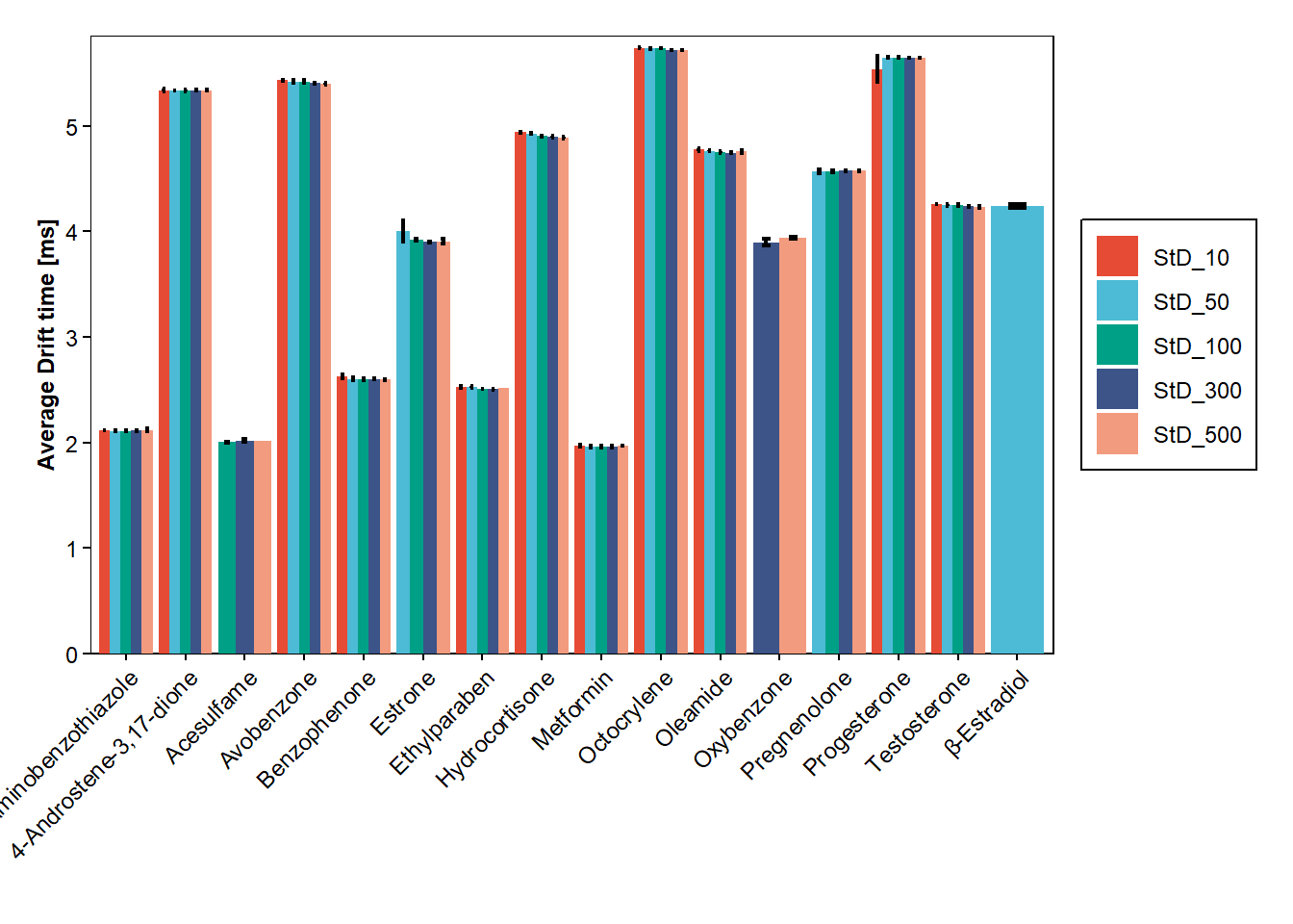

bar_plot(data_hrms_average, Compound, Average_CCS, Sample_Item, SEM_CCS)+
  labs(y = expression("Average CCS [Å"^"2"~"]"), x="")+
  scale_y_continuous(expand = expansion(add=c(0,10)))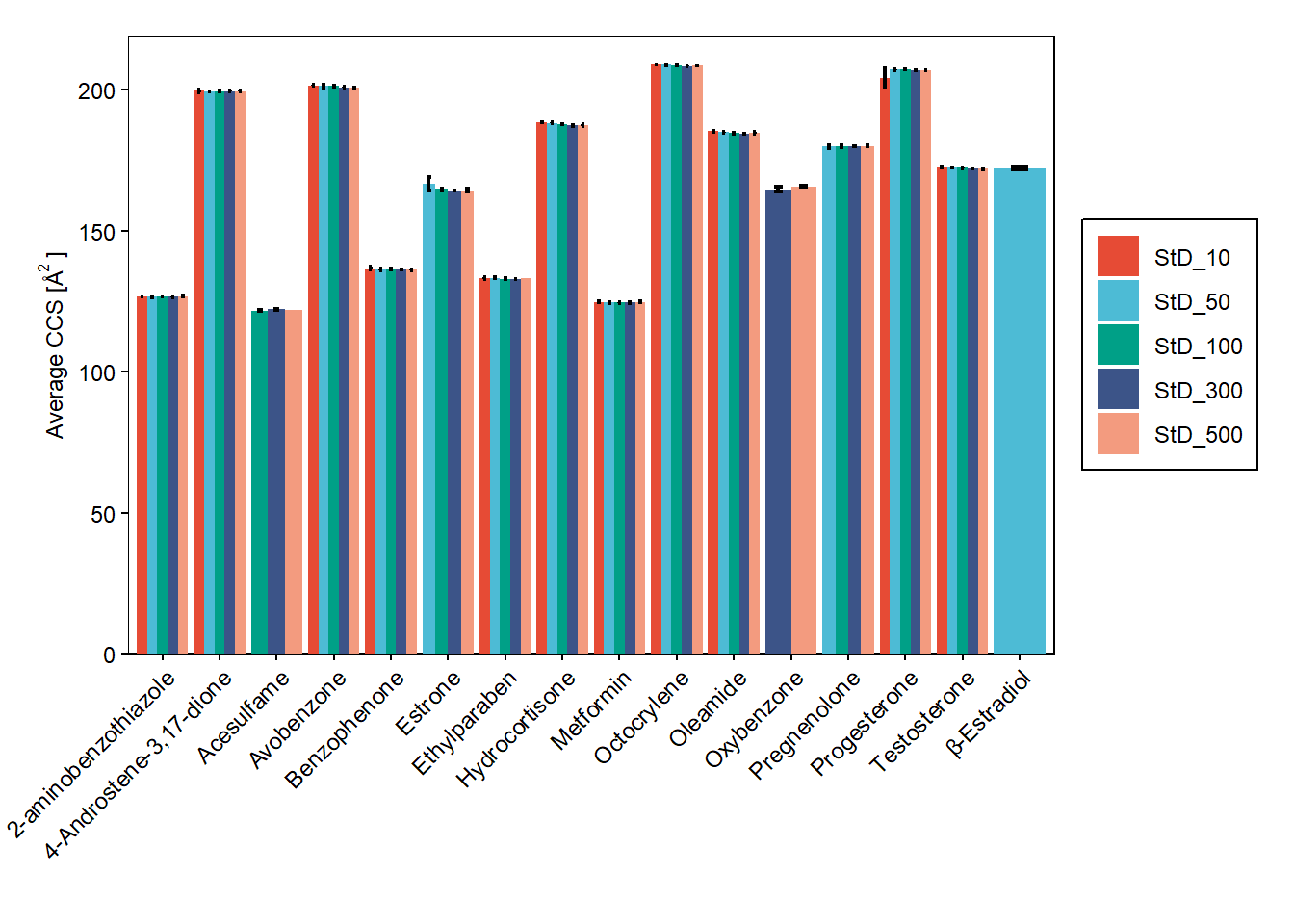

bar_plot(data_hrms_average, Compound, Average_intensity, Sample_Item, SEM_intensity)+
  labs(y = "Average Intensity", x="")+
  scale_y_continuous(expand = expansion(add=c(0,100)))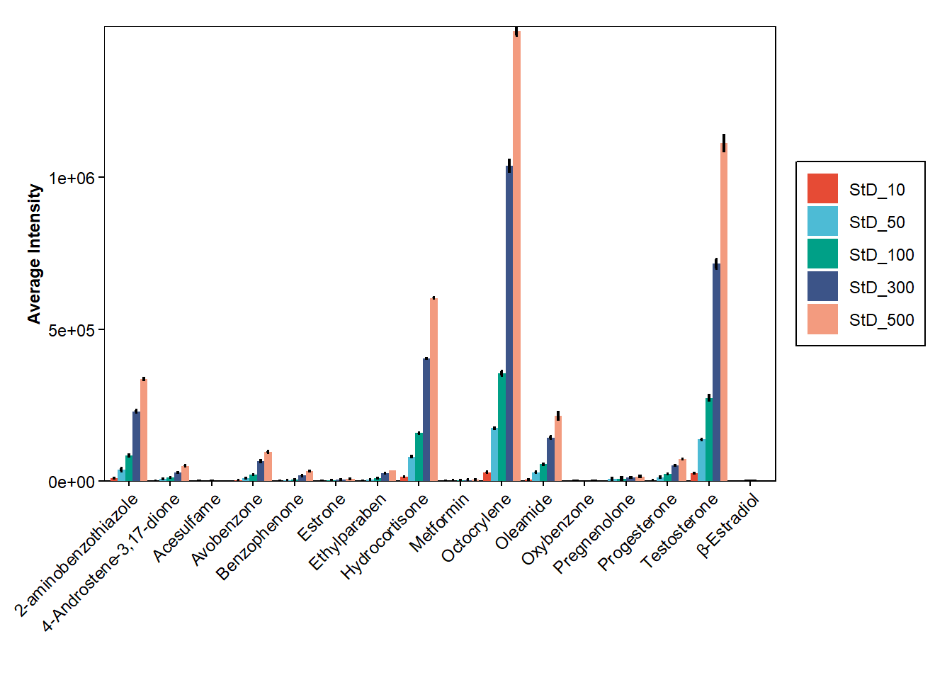

Plots using the scatter_plot function.

scatter_plot(data_hrms_average, Average_MZ, Average_RT, Compound, SEM_RT)+
  geom_text_repel(data=data_hrms_average |> distinct(Compound, .keep_all=TRUE),
                   aes(label=Compound),
                     size = 2.5,
                     point.padding = NA, # additional padding around each point
                     min.segment.length = 0, # draw all line segments
                     force=2,
                     nudge_x=3, nudge_y=0.1,
                     color="black"
                   )+
  labs(y = "Average Retention time [min]", x=expression(paste("Theoretical ",italic("m/z"), " values")))+
  theme(legend.position = "none")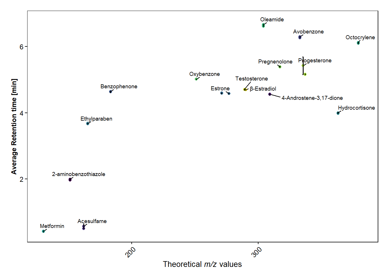

scatter_plot(data_hrms_average, Average_MZ, Average_CCS, Compound, SEM_CCS)+
  labs(y = "Average Drift time [min]", x=expression(paste("Theoretical ",italic("m/z"), " values")))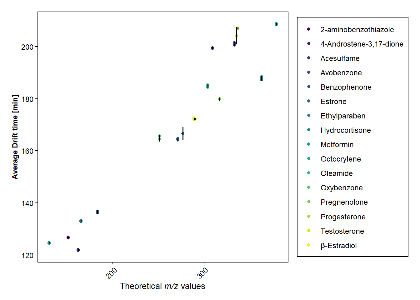

---

If measured samples are standards of different concentrations, calibration curves can be plotted.

Plotting calibration curves of the concentration vs intensities to be able to visually see the regression. However, to obtain the Standard Error of the Slope and the Slope for calculation of Limit of Detection (LOD), no calibration curve needs to be plotted.

#End of the Sample_Item-names contains the concentrations in ppb, which is added to a new column
data_hrms_average <- data_hrms_average |> 
  mutate(Concentration = as.numeric(str_extract(Sample_Item, "\\d+")))

#Plot the calibrations curves for each compounds in separate plots. To each calibration curve is the R^2 added
ggplot(data=data_hrms_average, mapping=aes(x=Concentration, y=Average_intensity, colour=Compound))+
  geom_errorbar(aes(ymin=Average_intensity-SEM_intensity, ymax=Average_intensity+SEM_intensity), width=3, size=0.6, colour="black")+
  geom_point() +
  geom_smooth(method="lm", 
              size=0.6, 
              se=FALSE, 
              linetype="dashed",
              fullrange=TRUE,
              aes(color=Compound))+ 
  stat_cor(aes(label=..rr.label..), label.x=200, size=3, colour="black", r.digits = 5)+ #adds R^2
  facet_wrap(~ Compound, scales="free")+ #separates the plots for each compound
  scale_color_viridis(discrete=TRUE)+
  theme_minimal()+
  theme(
    panel.background = element_rect(fill = "white"),  # Set white background
    panel.grid.major = element_blank(),  # Remove grid lines
    panel.grid.minor = element_blank(),  # Remove grid lines
    axis.text = element_text(size = 9),  # Increase font size of axis text
    axis.title.y = element_text(size = 9,face = "bold"),  # Make y-axis label bold and italic
    axis.text.y = element_text(color = "black", size = 9),  # Make x-axis text bold
    axis.title.x = element_text(size = 10,face = "bold"),
    axis.text.x = element_text(color = "black", size = 9),  # Make x-axis text bold
    axis.ticks.x = element_line(color = "black"),  # Add ticks to x-axis in black color
    axis.ticks.y = element_line(color = "black"),  # Add ticks to y-axis in black color
    plot.margin = margin(0.5, 0.5, 0.4, 0.5, "cm"),  # Set plot margins
    legend.position = "none"
)+
  labs(y = "Average Intensity", x="Concentration [ppb]")

Warning: The dot-dot notation (`..rr.label..`) was deprecated in ggplot2 3.4.0.
ℹ Please use `after_stat(rr.label)` instead.

`geom_smooth()` using formula = 'y ~ x'

Warning: Computation failed in `stat_cor()`.
Caused by error in `cor.test.default()`:
! not enough finite observations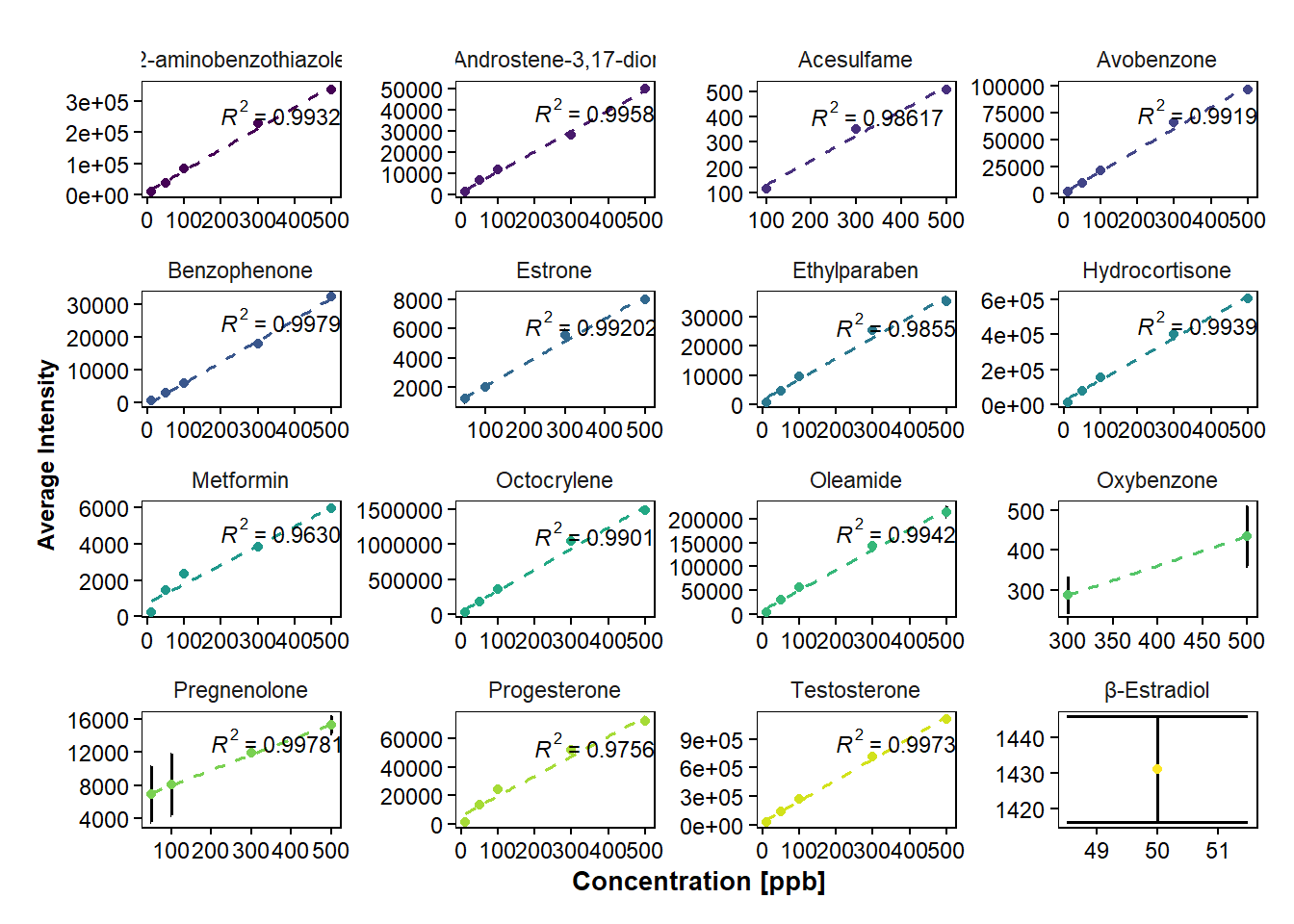

# Obtain the Slope (a) and Intercept (b) for each calibration curve (y=ax+b)
regression_1 <- data_hrms_average |> 
  group_by(Compound)  |> 
  do(tidy(lm(Average_intensity ~ Concentration, data = .)))  |> 
  filter(term %in% c("Concentration", "(Intercept)"))  |> 
  mutate(parameter = if_else(term == "Concentration", "Slope", "Intercept"))  |> 
  select(Compound, parameter, estimate)  |> 
  spread(parameter, estimate)

##### Obtain the Slope (a) for each calibration curve (y=ax+b)#####
#regression_1 <- data_hrms_average |> 
#  group_by(Compound) |> 
#  do(tidy(lm(Average_intensity ~ Concentration, data = .)))  |> 
#  filter(term == "Concentration")  |> 
#  select(Compound, Slope = estimate)

# Obtain the StDErrorY for each calibration curve
regression_2 <- data_hrms_average |> 
   group_by(Compound) |> 
   do(augment(lm(Average_intensity ~ Concentration, data = .))) |> 
   summarise(StdErrorY = sd(.resid))  |> 
   select(Compound, StdErrorY)
# Combines the two data frames with Slope and StDErrorY, and calculate the LOD and LOQ for them
regression_data_hrms_average <- regression_1 |> 
  inner_join(regression_2, join_by(Compound)) |>   
  mutate(`LOD_[ppb]`= round(3.3*StdErrorY/Slope,digits=3)) |> 
  mutate(`LOQ_[ppb]`= round(10*StdErrorY/Slope,digits=3))

#Calculate the concentration from the calibration curve for selected Sample_Item and Replicate

sample <- "StD_300"
nr_replicate <- 1

cal_conc_data_hrms <- data_hrms |> 
  filter(Sample_Item == sample & Replicate == nr_replicate) |>
  semi_join(regression_data_hrms_average, by = "Compound") |> 
  mutate(Calculated_Conc = cal_conc(Detector_Counts, regression_data_hrms_average$Intercept, regression_data_hrms_average$Slope))


#Create a table with the calculated concentrations
gt_tab <- cal_conc_data_hrms |> filter(!is.na(Calculated_Conc))|> 
  select(Compound, Mass_to_Charge_Ratio, Retention_Time, Drift_Time, CCS, Calculated_Conc) |> 
  gt() |>
  tab_options(table.font.color="black")|> 
  tab_header(
      title=md("**Calculated Concentrations**"), #**to make bold
      ) |> 
  fmt_number(columns = c(Mass_to_Charge_Ratio, Retention_Time, Drift_Time, CCS, Calculated_Conc), decimals=3) |>  #to formate numbers, can select specific columns to display certain nr. of deicmals for example. 
  cols_label(
    Mass_to_Charge_Ratio = md("*m/z*"),
    Retention_Time = md("Retention Time <br>[min]"),
    Drift_Time = md("Drift Time <br>[ms]"),
    CCS = md("Å^2^"),
    Calculated_Conc = md("Calculated Concentrations")
  ) 
gt_tab 

Calculated Concentrations
Compound	m/z	Retention Time [min]	Drift Time [ms]	Å2	Calculated Concentrations
2-aminobenzothiazole	151.031	1.970	2.110	126.520	318.219
4-Androstene-3,17-dione	309.181	4.560	5.330	199.330	280.012
Acesulfame	161.986	0.500	2.030	122.290	339.575
Avobenzone	333.144	6.270	5.410	201.040	346.053
Benzophenone	183.079	4.630	2.610	136.290	279.538
Estrone	271.168	4.590	3.900	164.320	354.133
Ethylparaben	165.055	3.680	2.510	132.870	335.132
Hydrocortisone	363.215	3.990	4.910	187.490	320.619
Metformin	130.107	0.430	1.970	124.750	310.067
Octocrylene	379.237	6.100	5.720	208.560	344.356
Oleamide	304.260	6.620	4.750	184.470	333.817
Oxybenzone	251.066	5.010	3.890	164.410	417.382
Pregnenolone	317.247	5.390	4.560	179.710	272.946
Progesterone	337.212	5.160	5.640	206.850	332.579
Testosterone	289.215	4.700	4.240	172.150	303.769

#gt_tab |> gtsave(filename = "tab_1.html") #saves the table in HTML format
#gt_tab |> gtsave(filename = "tab_1.tex") #saves the table in LaTEX format
#gt_tab |> gtsave(filename = "tab_1.docx") #saves the table in WORD format

---

4.4 Processed Data MS-DIAL

This section is for data that has been exported from UNIFI and then been processed in MS-DIAL. Hence, the output file contains many features and the target compounds needs to be extracted from the processed output file by comparison with expected data (e.g. theoretical m/z of different adducts).

Data_HRMS_Format_StDB_A <- read_excel("~/01_Projects/02_NM-CT-stdAB_Collaboration_CCS_MEASURMENT_2024/NMCTAB_2024_03_21_MSconvert_MSDIAL/Data_HRMS_Format_StDB.xlsx", 
    sheet = "Data_StDB_A_MSDIAL_1001_2")


Data_HRMS_Format_StDB_A |> mutate(diff_CCS = (`UNIFI ccs`-CCS)/`UNIFI ccs`*100) |> 
  ggplot(aes(x=Mass_to_Charge_Ratio, y=diff_CCS))+
  geom_point()

Warning: Removed 21 rows containing missing values or values outside the scale range
(`geom_point()`).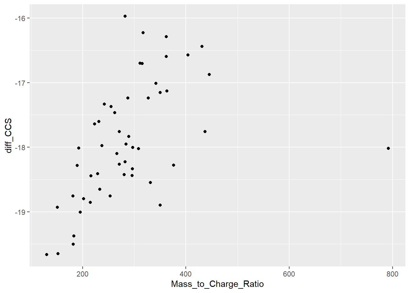

  #xlim(190,350)

ggplot(Data_HRMS_Format_StDB_A, aes(x=Mass_to_Charge_Ratio,y=CCS, label=Compound))+
  geom_point()+
  geom_point(aes(x=Mass_to_Charge_Ratio,y=`UNIFI ccs`, label=Compound), color="red")

Warning in geom_point(aes(x = Mass_to_Charge_Ratio, y = `UNIFI ccs`, label = Compound), : Ignoring unknown aesthetics: label
Removed 21 rows containing missing values or values outside the scale range
(`geom_point()`).
Removed 21 rows containing missing values or values outside the scale range
(`geom_point()`).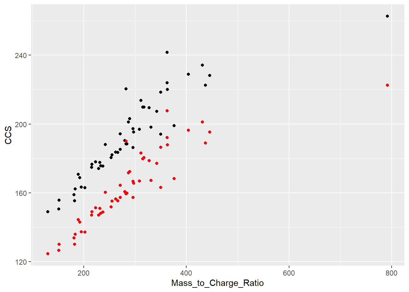

  geom_label_repel(size = 2.5,
                   point.padding = NA, # additional padding around each point
                   min.segment.length = 0, # draw all line segments
                   force=2,
                   fill= alpha("white",0),
                   nudge_x=2, nudge_y=2
                   )

geom_label_repel: parse = FALSE, box.padding = 0.25, label.padding = 0.25, point.padding = NA, label.r = 0.15, label.size = 0.25, min.segment.length = 0, arrow = NULL, na.rm = FALSE, force = 2, force_pull = 1, max.time = 0.5, max.iter = 10000, max.overlaps = 10, nudge_x = 2, nudge_y = 2, xlim = c(NA, NA), ylim = c(NA, NA), direction = both, seed = NA, verbose = FALSE
stat_identity: na.rm = FALSE
position_nudge_repel