#Data is importer for the two data set (mzmine and ms_dial). A reference data frame is constructed (unifi) as well as data frame with theoretical values (qc_compounds).

mzmine <- read_excel("C:/Users/vicer06/OneDrive - Linköpings universitet/Documents/01_Projects/01_VION_HRMS_MSConvert_Processing_2024/QC_mix_MSDIAL_MZmine_Files/qc5rep_hdmse_peakpicking_featurelist_MZMINE.xlsx",
    col_types = c("text", "text", "numeric",
        "numeric", "text", "text", "numeric",
        "numeric", "text", "numeric", "numeric",
        "text", "text", "text", "text", "text",
        "text", "text", "numeric", "text",
        "text", "text", "text", "text", "numeric",
        "text", "text", "text", "text", "text",
        "text", "text", "text", "text", "text",
        "text", "text", "text", "text", "text",
        "text", "text", "text", "numeric",
        "numeric", "numeric", "text", "text",
        "text", "text", "text", "text", "text",
        "text", "text", "text", "text", "text",
        "text", "text", "text", "text", "text",
        "text", "numeric", "numeric", "numeric",
        "text", "text", "text", "text", "text",
        "text", "text", "text", "text", "text",
        "text", "text", "text", "text", "text",
        "text", "text", "text", "numeric",
        "numeric", "numeric"))

ms_dial <- read_excel("C:/Users/vicer06/OneDrive - Linköpings universitet/Documents/01_Projects/01_VION_HRMS_MSConvert_Processing_2024/QC_mix_MSDIAL_MZmine_Files/qc3rep_hdmse_peakpicking_featurelist_MSDIAL.xlsx")

unifi <- data.frame(compound=c("acetaminophen","caffeine","leucine enkephaline","reserpine","sulfadimethoxine","sulfaguanidine","terfenadine","val-tyr-val","verapamil")
  , mz_unifi=c(152.0697, 195.0870, 556.2756, 609.2787, 311.0801, 215.0589, 472.3197, 380.2173, 455.2892),
  rt_unifi=c(0.56,1.30,2.37,3.37,2.96,0.31,3.66,1.28,3.26),
  dt_unifi=c(2.26,2.60,6.41,7.23,4.00,3.01,6.48,5.05,5.66))

qc_compounds <- data.frame(
  compound=c("acetaminophen","caffeine","leucine enkephaline","reserpine","sulfadimethoxine","sulfaguanidine","terfenadine","val-tyr-val","verapamil")
, mz=c(152.0705, 195.0876, 556.2765, 609.2806, 311.0808, 215.0597, 472.3209, 380.2179, 455.2904))3 Data Analysis
Some analysis of data. Most of the code is just to try different functions and methods to analyse data from a LC-IMS-HRMS instrument and to compare the processing of the data between different softwares.
3.1 QC mixture
The following part is for analysis of a QC mixture containing 9 analytes.
#Creating new objects with only the a subset of the data for both data sets. RT and Mobility is rounded to two digits to be compariable to unifi data

#Only keep the rows that corresponds to the compounds in qc_compounds for mzmine data set
mzmine_subset <- mzmine |>
  select(id,height,ion_mobility,rt,mz) |>  #to only include those columns in the new data frame
  mutate(across(c(rt,ion_mobility),round, 2)) |> #round the rt and ion mobility columns values to two decimals
  mutate(across(mz,round, 4)) |> #round the mz values to four decimals
  filter(id %in% qc_compounds$compound ) #only keeps the rows in id that is labeled as one of the compounds in qc_compounds data frame
Warning: There was 1 warning in `mutate()`.
ℹ In argument: `across(c(rt, ion_mobility), round, 2)`.
Caused by warning:
! The `...` argument of `across()` is deprecated as of dplyr 1.1.0.
Supply arguments directly to `.fns` through an anonymous function instead.
# Previously
across(a:b, mean, na.rm = TRUE)
# Now
across(a:b, \(x) mean(x, na.rm = TRUE))#msdial data is filtered to excluded the rows where mobility is -1.00 since those are duplicates
#Also only keep rows that corresponds to the qc compounds
msdial_subset <- ms_dial |>
select(`Alignment ID`,Average,`Average Rt(min)`,`Average mobility`,`Average Mz`) |>
mutate(across(c(`Average Rt(min)`,`Average mobility`),round, 2)) |>
mutate(across(`Average Mz`,round, 4)) |>
filter(`Average mobility` != -1.00 & `Alignment ID` %in% qc_compounds$compound )ALTERNATIVE METHOD FOR THE ABOVE WRITTEN CODE
The methods used above realize on that the “correct” compounds names have manually been added before to the data before importing it in RStudio. However, to skip having to manually add them, the following part is for finding the correct compounds in mzmine or msdial that corresponds to the ones in UNIFI/ QC_compounds data frame.
The criteria for a match is based on the retention time (RT), drift time (DT), and Mass-To-Charge ration(m/z) compared to the values in UNIFI.
- For doing this the
join-functions can be used.
| R for Data Science (2e) - 19 Joins (hadley.nz) |
“Mutating joins, which add new variables to one data frame from matching observations in another.” e.g. left_join() and inner_join() |
“Filtering joins, which filter observations from one data frame based on whether or not they match an observation in another.” e.g. semi_join() and anti_join() |
#First import the data (if the first code chunk have not been run for importing data
mzmine <- read_csv("C:/Users/vicer06/OneDrive - Linköpings universitet/Documents/01_Projects/01_VION_HRMS_MSConvert_Processing_2024/QC_mix_MSDIAL_MZmine_Files/qc5rep_hdmse_peakpicking_featurelist_MZMINE.csv",show_col_types = FALSE)
#glimpse(mzmine)
msdial <- ms_dial <- read_excel("C:/Users/vicer06/OneDrive - Linköpings universitet/Documents/01_Projects/01_VION_HRMS_MSConvert_Processing_2024/QC_mix_MSDIAL_MZmine_Files/qc3rep_hdmse_peakpicking_featurelist_MSDIAL.xlsx")

mzmine |> filter(is.na(rt) | is.na(mz) | is.na(ion_mobility)) #check that there are no missing values. Need to have entries for each obesrvation
# A tibble: 0 × 130
# ℹ 130 variables: id <dbl>, area <dbl>, ion_mobility <dbl>, rt <dbl>,
# mz_range:min <dbl>, mz_range:max <dbl>, charge <dbl>, fragment_scans <dbl>,
# alignment_scores:rate <dbl>, alignment_scores:aligned_features_n <dbl>,
# alignment_scores:align_extra_features <dbl>,
# alignment_scores:weighted_distance_score <dbl>,
# alignment_scores:mz_diff_ppm <dbl>, alignment_scores:mz_diff <dbl>,
# alignment_scores:rt_absolute_error <dbl>, …mzmine |> count(rt, mz, ion_mobility) |> filter(n>1) #check that the variables uniquely identifies each feature# A tibble: 0 × 4
# ℹ 4 variables: rt <dbl>, mz <dbl>, ion_mobility <dbl>, n <int>msdial |> filter(is.na(`Average Rt(min)`) | is.na(`Average Mz`) | is.na(`Average mobility`)) #check that there are no missing values. Need to have entries for each obesrvation# A tibble: 0 × 22
# ℹ 22 variables: Alignment ID <chr>, Average Rt(min) <dbl>, Average Mz <dbl>,
# Average mobility <dbl>, Average CCS <dbl>, Metabolite name <chr>,
# Adduct type <chr>, Post curation result <chr>, Fill % <dbl>,
# MS/MS assigned <lgl>, Annotation tag (VS1.0) <dbl>,
# Manually modified for quantification <lgl>,
# Manually modified for annotation <lgl>, S/N average <dbl>,
# Spectrum reference file name <chr>, MS1 isotopic spectrum <chr>, …msdial |> count(`Average Rt(min)`, `Average Mz`, `Average mobility`) |> filter(n>1) #check that the variables uniquely identifies each feature# A tibble: 0 × 4
# ℹ 4 variables: Average Rt(min) <dbl>, Average Mz <dbl>,
# Average mobility <dbl>, n <int>To combine two data frames by using the join -functions (left_join(), inner_join(), right_join(), full_join(), semi_join(), anti_join()) in dplyr -packages.
left_join(): output will have the same number of rows as input data frame x.
mzmine2 <- mzmine #copied the data frames only for testing purposes
unifi2 <- unifi
msdial2 <- msdial

#MsDial data does not have mz and rt ranges as MzMine data has, therefore added manually
msdial2$mz_min <- msdial2$`Average Mz`-0.005
msdial2$mz_max <- msdial2$`Average Mz`+0.005
msdial2$rt_min <- msdial2$`Average Rt(min)`-0.08
msdial2$rt_max <- msdial2$`Average Rt(min)`+0.08

#finds the compounds from unifi in the mzmine data by using the join function
subset_mzmine <- unifi2 |> inner_join(mzmine2, join_by(overlaps("mz_unifi","mz_unifi","mz_range:min", "mz_range:max"),overlaps("rt_unifi","rt_unifi","rt_range:min", "rt_range:max"))) |>
  filter(abs(dt_unifi - ion_mobility) < 2)

#subset_msdial <- unifi2 |> inner_join(msdial2, join_by(overlaps("mz_unifi","mz_unifi","mz_min", "mz_max"),overlaps("rt_unifi","rt_unifi","rt_min", "rt_max"))) |> filter(abs(dt_unifi - `Average mobility`) < 1.7)

#finds the compounds from unifi in the msdial data by using the join function
subset_msdial <- unifi2 |>
  inner_join(msdial2, join_by(overlaps("mz_unifi","mz_unifi","mz_min", "mz_max"),overlaps("rt_unifi","rt_unifi","rt_min", "rt_max"))) |>
  group_by(mz_unifi) |>
  mutate(dt_diff = abs(dt_unifi - `Average mobility`)) |>
  filter(dt_diff <=min(dt_diff))

no_duplicates_msdial <- subset_msdial[!duplicated(subset_msdial$compound), ] #removes the second duplicate feature
To easier be able to calculate the mass error, a function was created.
\(MassError[ppm]=\frac{\textit{m/z}_{theretical}-\mathit{m/z}_{measured}}{\mathit{m/z}_{theoretical}}*10^6\)
#function to calculate the mass error
mass_error <- function(mz_theoretical,mz_meaured){
  mass_error <- (mz_theoretical-mz_meaured)/mz_theoretical*10^6
  return(mass_error)
}

mass_error(qc_compounds$mz,subset_mzmine$mz)
[1] 4.668887 2.921764 2.480781 4.989491 2.218073 2.324936 3.366355 4.891932
[9] 2.174436mass_error(qc_compounds$mz,no_duplicates_msdial$`Average Mz`)[1] 3.6167435 0.6151083 1.0066936 0.1313024 2.4109492 0.7439795 2.0748605
[8] 2.7352736 0.4612441The following part is used with the “first method” of extracting the correct compounds from msdial and mzmine because ti was written before the other method was written. Sorry for the mess in jumping between different parts.
#calculate the mass accuracy for mzmine, msdial, and unif based on the qc_compounds values. First the m/z values are sorted from small to large so the calculations can be performed row-wise for the correct compound in QC_compounds and the data. Lastly, the results are added to a column in a new object.

qc_compounds <- arrange(qc_compounds, mz)
mass_errors <- as.data.frame(qc_compounds[1:2]) #create an data frame to add all the mass errors to

#calculate mass errors
mzmine_subset <- mzmine_subset |> arrange(mz) |> mutate(Mass_error_ppm = round((qc_compounds$mz-mz)/qc_compounds$mz*10^6,3))
msdial_subset <- msdial_subset |> arrange(`Average Mz`) |> mutate(Mass_error_ppm = round((qc_compounds$mz - `Average Mz`) /qc_compounds$mz * 10^6,3))
unifi <- unifi |> arrange(mz_unifi) |> mutate(Mass_error_ppm = round((qc_compounds$mz - mz_unifi) /qc_compounds$mz * 10^6,3))

#adds the mass errors to the mass error data frame
mass_errors$Mzmine <- mzmine_subset$Mass_error_ppm
mass_errors$MsDial <- msdial_subset$Mass_error_ppm
mass_errors$Unifi <- unifi$Mass_error_ppm

#Adds a column that tells if the Mzmine or MsDial Mass errors are close or far away from the error of Unifi
mass_errors <- mass_errors |> mutate(mzmine_fromunifi = case_when(abs(Unifi - Mzmine) > 2 ~ "Large",
                                                   abs(Unifi - Mzmine) <= 2 & abs(Unifi - Mzmine) > 0.3 ~ "Medium",
                                                   abs(Unifi - Mzmine) <= 0.3 ~ "Small")) |>
  mutate(msdial_fromunifi = case_when(abs(Unifi - MsDial) > 2 ~ "Large",
                                                   abs(Unifi - MsDial) <= 2 & abs(Unifi - MsDial) > 0.3 ~ "Medium",
                                                   abs(Unifi - MsDial) <= 0.3 ~ "Small"))
Next parts of chunks are for plotting the data for the QC compounds.
#Plot the mass errors towards the theoretical m/z values
mass_errors$msdial_fromunifi <- as.factor(mass_errors$msdial_fromunifi)
mass_errors$mzmine_fromunifi <- as.factor(mass_errors$mzmine_fromunifi)

p <- ggplot(data=mass_errors, mapping=aes(x=mz))+
  geom_point(aes(y=Mzmine, colour="Mzmine", shape="Mzmine", size=mzmine_fromunifi), alpha = 0.7)+ #mass erros values from mzmine and adds size of the plots according to how far away they are from unifi
  geom_point(aes(y=MsDial, colour="MsDial", shape="MsDial", size=msdial_fromunifi), alpha = 0.7)+ #mass erros values from msdial and adds size of the plots according to how far away they are from unifi
  geom_line(aes(y=Unifi, colour="Unifi"),size=0.5)+ #plot Unifi data

  scale_size_manual(name="Distance from Unifi", values = c("Large"=4.2, "Medium"=2.8, "Small"=2))+
  scale_shape_manual(values = c("Mzmine" = 19, "MsDial" = 17)) +
  scale_colour_manual(values = c("Mzmine" = "darkred", "MsDial" = "black", "Unifi" = "darkgrey")) + #colours of points
  labs(fill = "", y = "Mass Accuracy [ppm]", x=expression(paste("Theoretical ",italic("m/z"), " values"))) +

  geom_hline(yintercept = 0, linetype = "dashed", color = "red", linewidth = 0.1) + #adds horzontal line at y=0

  theme_minimal()+
  theme(
    panel.background = element_rect(fill = "white"),  # Set white background
    panel.grid = element_blank(),  # Remove grid lines
    axis.text = element_text(size = 9),  # Increase font size of axis text
    axis.title.y = element_text(size = 9,face = "bold"),  # Make y-axis label bold and italic
    axis.text.y = element_text(color = "black", size = 9),  # Make x-axis text bold
    axis.title.x = element_text(size = 10,face = "bold"),
    axis.text.x = element_text(color = "black", size = 9),  # Make x-axis text bold
    axis.ticks.x = element_line(color = "black"),  # Add ticks to x-axis in black color
    axis.ticks.y = element_line(color = "black"),  # Add ticks to y-axis in black color
    aspect.ratio = 0.5,  # Set aspect ratio
    plot.margin = margin(0.5, 0.5, 0.4, 0.5, "cm"),  # Set plot margins
    legend.text=element_text(size=9),
    legend.position = "right",
    legend.background = element_rect(fill="white",
                                   size=0.5, linetype="solid",
                                   colour ="black"),
    #legend.title = element_blank(), #removes the title of the legend
    legend.title = element_text(size=9),
    legend.margin = margin(0.001, 1, 0.5, 0.5),)
Warning: Using `size` aesthetic for lines was deprecated in ggplot2 3.4.0.
ℹ Please use `linewidth` instead.Warning: The `size` argument of `element_rect()` is deprecated as of ggplot2 3.4.0.
ℹ Please use the `linewidth` argument instead.p + geom_text(aes(x=mz+10, y=Unifi,label=compound), size=2, colour="red4",
nudge_x = 0.25, nudge_y = 0.25,
check_overlap = FALSE) #adds a text for the mean point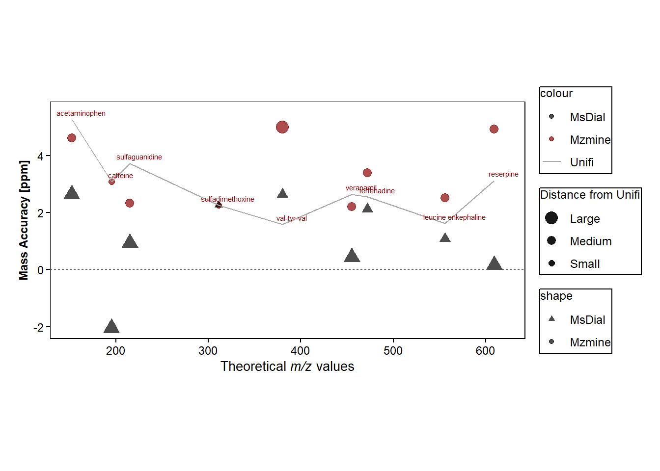
#+ guides(size = "none")#RT and DT difference between MS-Dial and Mzmine compared to UNIFI
#adding and then renaming the RT columns from each file
rt_difference <- data.frame(qc_compounds[,], msdial_subset[,3], mzmine_subset[,4], unifi[,3]) |> rename(MsDial_RT="Average.Rt.min.", MzMine_RT="rt", Unifi_RT="unifi...3.")
#adding and then renaming the DT columns from each file
dt_difference <- data.frame(qc_compounds[,], msdial_subset[,4], mzmine_subset[,3], unifi[,4]) |> rename(MsDial_DT="Average.mobility", MzMine_DT="ion_mobility", Unifi_DT="unifi...4.")
dt_difference <- dt_difference |>
mutate("diff_msdial" = MsDial_DT - Unifi_DT) |>
mutate("diff_mzmine" = MzMine_DT - Unifi_DT)
#rt_difference <- rt_difference |> mutate(mzmine_fromunifi = case_when(abs(Unifi - Mzmine) > 2 ~ "Large",
# abs(Unifi_RT - MzMine_RT) <= 2 & abs(Unifi_RT - MzMine_RT) > 0.3 ~ "Medium",
# abs(Unifi_RT - MzMine_RT) <= 0.3 ~ "Small")) |> mutate(msdial_fromunifi = case_when(abs(Unifi_RT - MsDial_RT) > 2 ~ "Large",
# abs(Unifi_RT - MsDial_RT) <= 2 & abs(Unifi_RT - MsDial_RT) > 0.3 ~ "Medium",
# abs(Unifi_RT - MsDial_RT) <= 0.3 ~ "Small"))
rt_difference_long <- rt_difference |> pivot_longer(cols = 3:5,
names_to = "Software",
values_to = "RT_softwares")
dt_difference_long <- dt_difference |> pivot_longer(cols = 3:5,
names_to = "software_name",
values_to = "DT_softwares") rt_difference_long |> filter(Software != "MsDial_RT" & Software != "MzMine_RT")# A tibble: 9 × 4
compound mz Software RT_softwares
<chr> <dbl> <chr> <dbl>
1 acetaminophen 152. Unifi_RT 0.56
2 caffeine 195. Unifi_RT 1.3
3 sulfaguanidine 215. Unifi_RT 0.31
4 sulfadimethoxine 311. Unifi_RT 2.96
5 val-tyr-val 380. Unifi_RT 1.28
6 verapamil 455. Unifi_RT 3.26
7 terfenadine 472. Unifi_RT 3.66
8 leucine enkephaline 556. Unifi_RT 2.37
9 reserpine 609. Unifi_RT 3.37#Plot of RT vs theoretical m/z values for the different softwares
b <- ggplot(data=rt_difference_long, mapping=aes(x=mz, y=RT_softwares))+
geom_bar(stat = "identity",position=position_dodge(), aes(fill=Software))+
scale_fill_manual(values = c("MzMine_RT" = "darkred", "MsDial_RT" = "darkgreen", "Unifi_RT" = "darkgrey")) + #colours of points
labs( y = "Retention time [min]", x=expression(paste("Theoretical ",italic("m/z"), " values"))) +
scale_y_continuous(limit=c(0,4),expand = c(0,0))+
#geom_text(aes(x=mz, y=RT_softwares, label=compound), size=2, colour="red4",
# nudge_x = 0.25, nudge_y = 0.25,
# check_overlap = FALSE)+
theme_minimal()+
theme(
panel.background = element_rect(fill = "white"), # Set white background
panel.grid.major = element_blank(), # Remove grid lines
panel.grid.minor = element_blank(), # Remove grid lines
axis.text = element_text(size = 9), # Increase font size of axis text
axis.title.y = element_text(size = 9,face = "bold"), # Make y-axis label bold and italic
axis.text.y = element_text(color = "black", size = 9), # Make x-axis text bold
axis.title.x = element_text(size = 10,face = "bold"),
axis.text.x = element_text(color = "black", size = 9), # Make x-axis text bold
axis.ticks.x = element_line(color = "black"), # Add ticks to x-axis in black color
axis.ticks.y = element_line(color = "black"), # Add ticks to y-axis in black color
#aspect.ratio = 1, # Set aspect ratio
plot.margin = margin(0.5, 0.5, 0.4, 0.5, "cm"), # Set plot margins
legend.text=element_text(size=9),
#legend.position = c(0.85, 0.85),
legend.background = element_rect(fill="white",
size=0.5, linetype="solid",
colour ="black"),
legend.title = element_blank(),
#legend.margin = margin(0.001, 1, 0.5, 0.5)
)
b + geom_label(data=rt_difference, mapping=aes(x=mz, y=MsDial_RT, label=compound),
size=2, colour="black",
nudge_x = 0.25, nudge_y = 0.15) 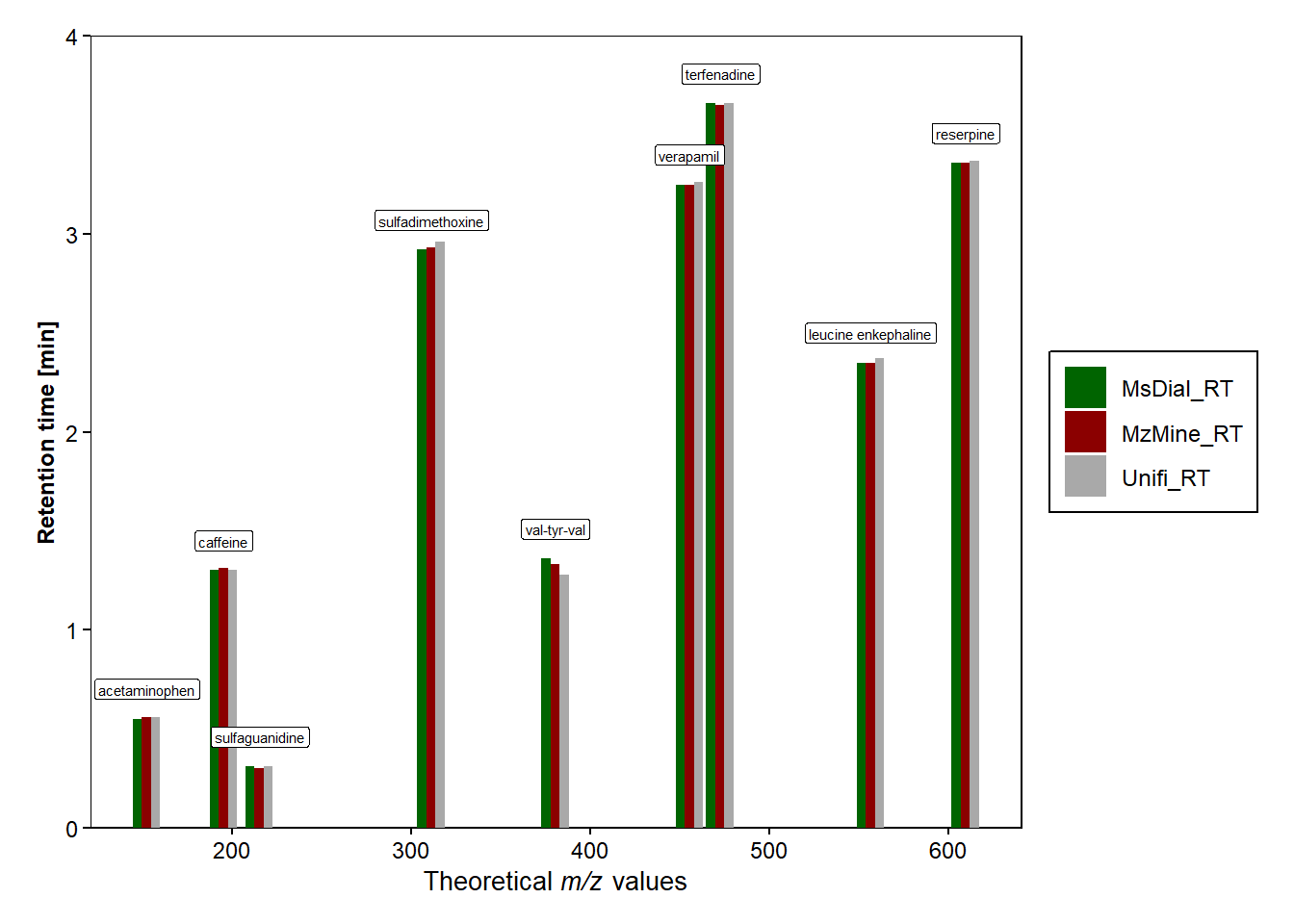
#Plot of DT vs theoretical m/z values for the different softwares
d <- ggplot(data=dt_difference_long, mapping=aes(x=mz, y=DT_softwares))+
  geom_bar(stat = "identity",position=position_dodge(), aes(fill=software_name))+

  scale_fill_manual(values = c("MzMine_DT" = "darkred", "MsDial_DT" = "darkgreen", "Unifi_DT" = "darkgrey")) +
  labs( y = "Drift Time [ms]", x=expression(paste("Theoretical ",italic("m/z"), " values"))) +
  scale_y_continuous(limit=c(0,10),expand = c(0,0))+ #removes the gap between the bars and the x-axis


  geom_line(data=dt_difference, color="black", aes(x=mz, y=Unifi_DT),size = 0.5, linetype = "dashed")+ #plots black line for Unifi_DT

  theme_minimal()+
  theme(
    panel.background = element_rect(fill = "white"),  # Set white background
    panel.grid.major = element_blank(),  # Remove grid lines
    panel.grid.minor = element_blank(),  # Remove grid lines
    axis.text = element_text(size = 9),  # Increase font size of axis text
    axis.title.y = element_text(size = 9,face = "bold"),  # Make y-axis label bold and italic
    axis.text.y = element_text(color = "black", size = 9),  # Make x-axis text bold
    axis.title.x = element_text(size = 10,face = "bold"),
    axis.text.x = element_text(color = "black", size = 9),  # Make x-axis text bold
    axis.ticks.x = element_line(color = "black"),  # Add ticks to x-axis in black color
    axis.ticks.y = element_line(color = "black"),  # Add ticks to y-axis in black color
    plot.margin = margin(0.5, 0.5, 0.4, 0.5, "cm"),  # Set plot margins
    legend.text=element_text(size=9),
    legend.background = element_rect(fill="white",
                                   size=0.5, linetype="solid",
                                   colour ="black"),
    legend.title = element_blank(),
)

d + geom_label(data=dt_difference, mapping=aes(x=mz-10, y=MzMine_DT, label=compound),
              size=2, colour="black", nudge_y = 0.7,
              ) #hjust="inward"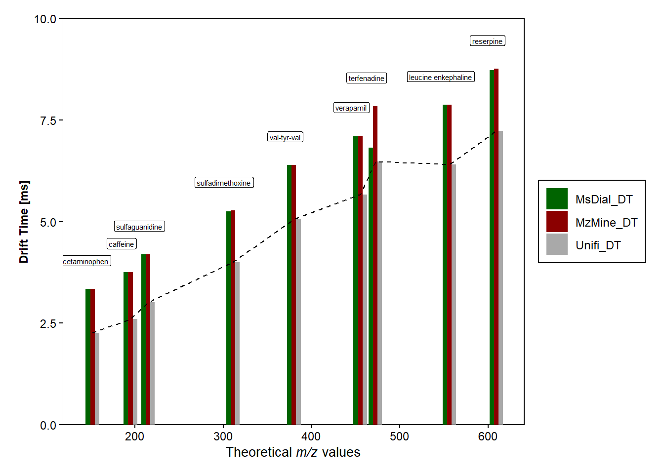
d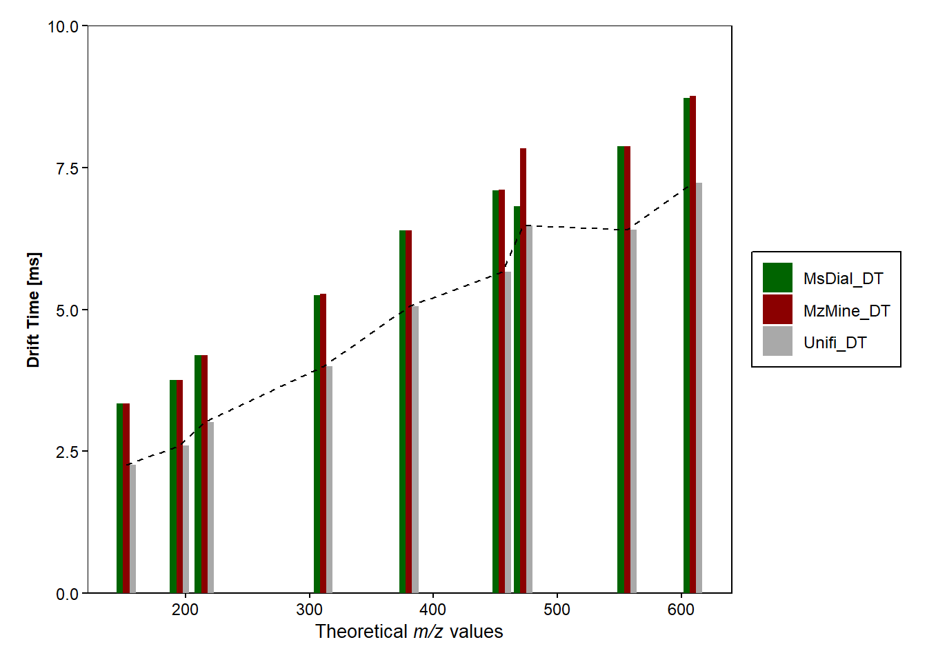
#Plot DT only for MSDial and adds regression line
d1 <- dt_difference |> filter(diff_msdial>0.5) |> #exlucde "outlier"
  ggplot(mapping=aes(x=mz, y=diff_msdial))+
  geom_point(size=1)+
  geom_smooth(method="loess", size=0.6, se=FALSE, linetype="dashed", color="darkred")+
  stat_cor(aes(label=..rr.label..), label.x=400, label.y=1.2, size=3, colour="black", r.digits = 5)+ #adds R^2
  theme_minimal()+
  theme(
    panel.background = element_rect(fill = "white"),  # Set white background
    panel.grid = element_blank(),  # Remove grid lines
    axis.text = element_text(size = 9),  # Increase font size of axis text
    axis.title.y = element_text(size = 9,face = "bold"),  # Make y-axis label bold and italic
    axis.text.y = element_text(color = "black", size = 9),  # Make x-axis text bold
    axis.title.x = element_text(size = 10,face = "bold"),
    axis.text.x = element_text(color = "black", size = 9),  # Make x-axis text bold
    axis.ticks.x = element_line(color = "black"),  # Add ticks to x-axis in black color
    axis.ticks.y = element_line(color = "black"),  # Add ticks to y-axis in black color
    aspect.ratio = 1,  # Set aspect ratio
    plot.margin = margin(0.5, 0.5, 0.4, 0.5, "cm"),  # Set plot margins
    legend.text=element_text(size=9),
    legend.position = c(0.25, 0.85),
    legend.background = element_rect(fill="white",
                                   size=0.5, linetype="solid",
                                   colour ="black"),
    legend.title = element_blank(), #removes the title of the legend
    legend.margin = margin(0.001, 1, 0.5, 0.5))
Warning: A numeric `legend.position` argument in `theme()` was deprecated in ggplot2
3.5.0.
ℹ Please use the `legend.position.inside` argument of `theme()` instead.d1Warning: The dot-dot notation (`..rr.label..`) was deprecated in ggplot2 3.4.0.
ℹ Please use `after_stat(rr.label)` instead.`geom_smooth()` using formula = 'y ~ x'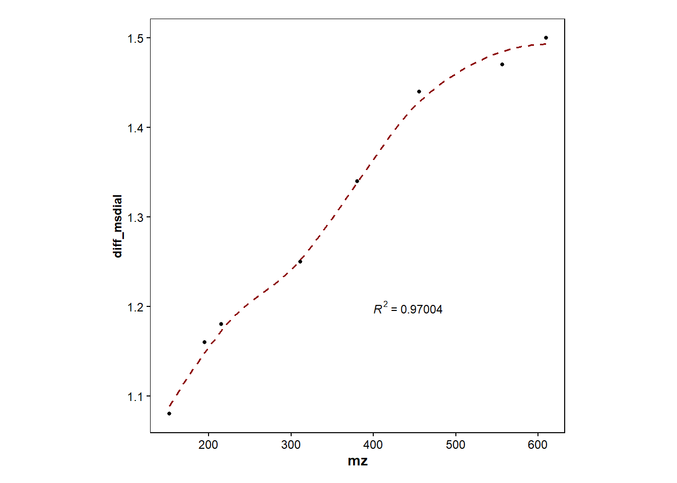
#Plot DT only for Mzmine and adds regression line
d2 <- dt_difference |> filter(compound != "terfenadine") |>
  ggplot(mapping=aes(x=mz, y=diff_mzmine))+
  geom_point(size=1)+
  geom_smooth(method="loess", size=0.6, se=FALSE, linetype="dashed", color="darkgreen")+
  stat_cor(aes(label=..rr.label..), label.x=200, label.y=1.4, size=3, colour="black", r.digits = 5)+ #adds R^2
  theme_minimal()+
  theme(
    panel.background = element_rect(fill = "white"),  # Set white background
    panel.grid = element_blank(),  # Remove grid lines
    axis.text = element_text(size = 9),  # Increase font size of axis text
    axis.title.y = element_text(size = 9,face = "bold"),  # Make y-axis label bold and italic
    axis.text.y = element_text(color = "black", size = 9),  # Make x-axis text bold
    axis.title.x = element_text(size = 10,face = "bold"),
    axis.text.x = element_text(color = "black", size = 9),  # Make x-axis text bold
    axis.ticks.x = element_line(color = "black"),  # Add ticks to x-axis in black color
    axis.ticks.y = element_line(color = "black"),  # Add ticks to y-axis in black color
    aspect.ratio = 1,  # Set aspect ratio
    plot.margin = margin(0.5, 0.5, 0.4, 0.5, "cm"),  # Set plot margins
    legend.text=element_text(size=9),
    legend.position = c(0.25, 0.85),
    legend.background = element_rect(fill="white",
                                   size=0.5, linetype="solid",
                                   colour ="black"),
    legend.title = element_blank(), #removes the title of the legend
    legend.margin = margin(0.001, 1, 0.5, 0.5))
d2
`geom_smooth()` using formula = 'y ~ x'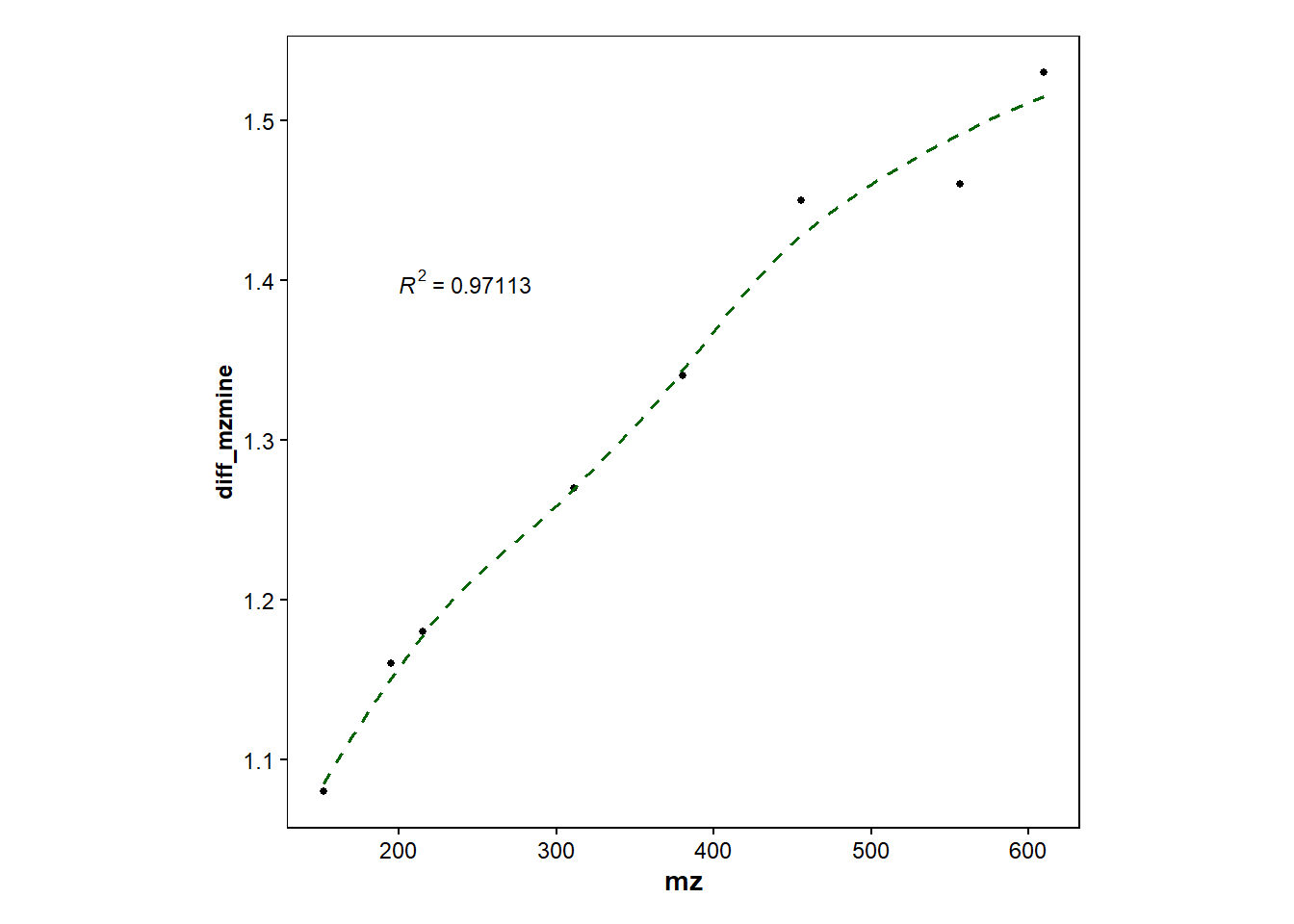
#Show both Mzmine and Msdial
ggarrange(d1, d2,
          labels = c("A", "B"),
          #ncol = 1, nrow = 2,
          widths = 2, heights = 10)
`geom_smooth()` using formula = 'y ~ x'
`geom_smooth()` using formula = 'y ~ x'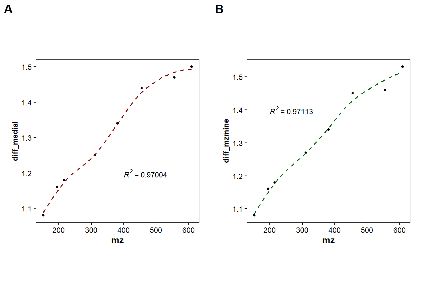
3.2 Drug mixture
The data used for this section is of a mixture of different drugs (200 ppb) including some Isotopically labeled internal standards (IS, 100 ppb). The data has been measured in ESI(+)-LC-IMS-HRMS (MSe mode, HDMSe) with different settings, here called old and new settings where the later is supposed to be more suitable for labile compounds. The data was processed in MZmine.
#Import the data from mzmine, and the excel sheet containing the target compounds and IS compounds.
data_drugmix <- read_csv("C:/Users/vicer06/OneDrive - Linköpings universitet/Documents/01_Projects/01_VION_HRMS_MSConvert_Processing_2024/QC_mix_MSDIAL_MZmine_Files/new_old_settings_drugmix_featurelist_MzMine.csv", show_col_types = FALSE) |>
  select(-`charge`,-`fragment_scans`,-`alignment_scores:rate`, -`alignment_scores:aligned_features_n`,-`alignment_scores:align_extra_features`,-`alignment_scores:weighted_distance_score`,-`alignment_scores:mz_diff_ppm`,-`alignment_scores:mz_diff`,-`alignment_scores:rt_absolute_error`,-`alignment_scores:ion_mobility_absolute_error`,-`intensity_range:min`,-`intensity_range:max`)

target_drugs <- read_excel("C:/Users/vicer06/OneDrive - Linköpings universitet/Documents/01_Projects/01_VION_HRMS_MSConvert_Processing_2024/Illicit_Drugs_Files/illicit drugs CS-IS_data.xlsx", na = "NA") |>
  filter(Class=="Analyte") |>
  mutate(rt_target_min = Vion_RT - 0.05) |>
  mutate(rt_target_max = Vion_RT + 0.05) |>
  select(-`Monoisomass`, -`Adduct_ion`,  -`Vion_observed_mz`, -`Agilent_observed_mz`, -`Agilent_RT`)


#find the target compounds in the drug_mix data
found_drugs <- target_drugs |> inner_join(data_drugmix, join_by(overlaps("Theor_adduct_mz","Theor_adduct_mz","mz_range:min", "mz_range:max"))) |>
  select(1:11, mz, height, everything()) #reorder columns

filtered_found_drugs <-found_drugs |> filter(
  !(`height` < 500), #removes rows with height less than 500
  !(!is.na(Vion_RT) & ("rt" < "rt_target_min" & "rt" > "rt_target_max")) #for those with prev. measured RT, compares them with currect RT
) |>
  slice_max(by=Compound, height) #to remove multiple features assigned the same compound by only keeping the ones with largest height. Due to not having any DT values to compare to filter the data more


#calculate the mass error and height and area ratio between new and old data
filtered_found_drugs <- filtered_found_drugs |>
  mutate(Mass_error_ppm = mass_error(Theor_adduct_mz, mz), .after = "mz")|>  #adds the mass error (calculated with the function) to a new column after m/z values
  mutate(height_ratio = `datafile:Drugdtd-200ppb-newsetting_1_A,2_1.mzML:height`/`datafile:Drugstd-200ppb_1_A,3_1.mzML:height`, .after="height") |> #adds the ratio between the height of the old and new settings
  mutate(area_ratio = `datafile:Drugdtd-200ppb-newsetting_1_A,2_1.mzML:area`/`datafile:Drugstd-200ppb_1_A,3_1.mzML:area`, .after="area") |>
  mutate(diff_DT = ion_mobility - DT_UNIFI, .after="ion_mobility") #different in ion mobility for the processed data compared to UNIFI


p1 <-ggplot(filtered_found_drugs, mapping = aes(x=mz, y=area_ratio, label=Compound))+ #plot area ratio
  geom_point()+
  geom_hline(yintercept = 1, linetype = "dashed", color = "red", linewidth = 0.1) + #adds horzontal line at y=0

  geom_label_repel(size = 2.5,
                   point.padding = NA, # additional padding around each point
                   min.segment.length = 0, # draw all line segments
                   force=2,
                   nudge_x=5, nudge_y=-0.03
                   )+

  theme_minimal()+
  theme(
    panel.background = element_rect(fill = "white"),  # Set white background
    panel.grid.major = element_blank(),  # Remove grid lines
    panel.grid.minor = element_blank(),  # Remove grid lines
    axis.text = element_text(size = 9),  # Increase font size of axis text
    axis.title.y = element_text(size = 9,face = "bold"),  # Make y-axis label bold and italic
    axis.text.y = element_text(color = "black", size = 9),  # Make x-axis text bold
    axis.title.x = element_text(size = 10,face = "bold"),
    axis.text.x = element_text(color = "black", size = 9),  # Make x-axis text bold
    axis.ticks.x = element_line(color = "black"),  # Add ticks to x-axis in black color
    axis.ticks.y = element_line(color = "black"),  # Add ticks to y-axis in black color
    plot.margin = margin(0.5, 0.5, 0.4, 0.5, "cm"),  # Set plot margins
    legend.text=element_text(size=9),
    legend.background = element_rect(fill="white",
                                   size=0.5, linetype="solid",
                                   colour ="black"),
    legend.title = element_blank(),
)
p2 <- ggplot(filtered_found_drugs, mapping=aes(x=mz,y=height_ratio,label=Compound))+ #plot height ratio
  geom_point()+
  geom_hline(yintercept = 1, linetype = "dashed", color = "red", linewidth = 0.1) + #adds horzontal line at y=0

  geom_label_repel(size = 2.5,
                   point.padding = NA, # additional padding around each point
                   min.segment.length = 0, # draw all line segments
                   force=2,
                   nudge_x=5, nudge_y=-0.03
                   )+

  theme_minimal()+
  theme(
    panel.background = element_rect(fill = "white"),  # Set white background
    panel.grid.major = element_blank(),  # Remove grid lines
    panel.grid.minor = element_blank(),  # Remove grid lines
    axis.text = element_text(size = 9),  # Increase font size of axis text
    axis.title.y = element_text(size = 9,face = "bold"),  # Make y-axis label bold and italic
    axis.text.y = element_text(color = "black", size = 9),  # Make x-axis text bold
    axis.title.x = element_text(size = 10,face = "bold"),
    axis.text.x = element_text(color = "black", size = 9),  # Make x-axis text bold
    axis.ticks.x = element_line(color = "black"),  # Add ticks to x-axis in black color
    axis.ticks.y = element_line(color = "black"),  # Add ticks to y-axis in black color
    plot.margin = margin(0.5, 0.5, 0.4, 0.5, "cm"),  # Set plot margins
    legend.text=element_text(size=9),
    legend.background = element_rect(fill="white",
                                   size=0.5, linetype="solid",
                                   colour ="black"),
    legend.title = element_blank(),
)

ggarrange(p1, p2,
          labels = c("A", "B"),
          #ncol = 1, nrow = 2,
          widths = 2, heights = 10)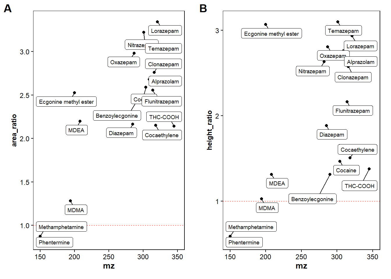
#Plot of DT difference between MZmine and UNIFI
p3 <- filtered_found_drugs |>
  ggplot(mapping=aes(x=Theor_adduct_mz, y=diff_DT))+
  geom_point(size=1)+
  geom_smooth(method="loess", size=0.6, se=FALSE, linetype="dashed", color="darkblue")+
  stat_cor(aes(label=..rr.label..), label.x=200, label.y=1.2, size=3, colour="black", r.digits = 5)+ #adds R^2

  theme_minimal()+
  theme(
    panel.background = element_rect(fill = "white"),  # Set white background
    panel.grid = element_blank(),  # Remove grid lines
    axis.text = element_text(size = 9),  # Increase font size of axis text
    axis.title.y = element_text(size = 9,face = "bold"),  # Make y-axis label bold and italic
    axis.text.y = element_text(color = "black", size = 9),  # Make x-axis text bold
    axis.title.x = element_text(size = 10,face = "bold"),
    axis.text.x = element_text(color = "black", size = 9),  # Make x-axis text bold
    axis.ticks.x = element_line(color = "black"),  # Add ticks to x-axis in black color
    axis.ticks.y = element_line(color = "black"),  # Add ticks to y-axis in black color
    aspect.ratio = 1,  # Set aspect ratio
    plot.margin = margin(0.5, 0.5, 0.4, 0.5, "cm"),  # Set plot margins
    legend.text=element_text(size=9),
    legend.position = c(0.25, 0.85),
    legend.background = element_rect(fill="white",
                                   size=0.5, linetype="solid",
                                   colour ="black"),
    legend.title = element_blank(), #removes the title of the legend
    legend.margin = margin(0.001, 1, 0.5, 0.5))
p3
`geom_smooth()` using formula = 'y ~ x'Warning: Removed 3 rows containing non-finite outside the scale range
(`stat_smooth()`).Warning: Removed 3 rows containing non-finite outside the scale range
(`stat_cor()`).Warning: Removed 3 rows containing missing values or values outside the scale range
(`geom_point()`).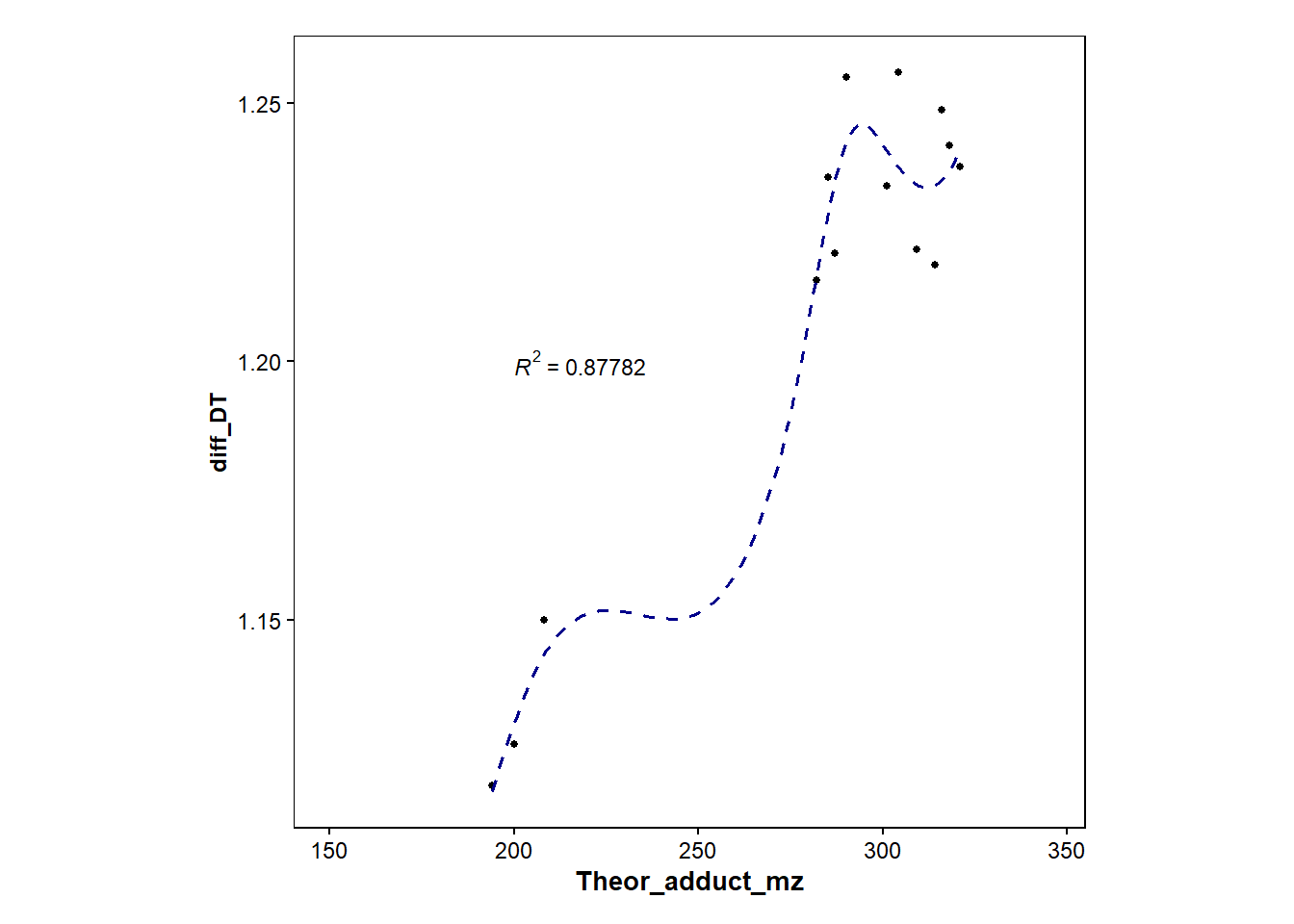
p4 <- filtered_found_drugs |>
  ggplot(mapping=aes(x=DT_UNIFI, y=diff_DT))+
  geom_point(size=1)+
  geom_smooth(method="loess", size=0.6, se=FALSE, linetype="dashed", color="orange")+
  stat_cor(aes(label=..rr.label..), label.x=4, label.y=1.2, size=3, colour="black", r.digits = 5)+ #adds R^2

  theme_minimal()+
  theme(
    panel.background = element_rect(fill = "white"),  # Set white background
    panel.grid = element_blank(),  # Remove grid lines
    axis.text = element_text(size = 9),  # Increase font size of axis text
    axis.title.y = element_text(size = 9,face = "bold"),  # Make y-axis label bold and italic
    axis.text.y = element_text(color = "black", size = 9),  # Make x-axis text bold
    axis.title.x = element_text(size = 10,face = "bold"),
    axis.text.x = element_text(color = "black", size = 9),  # Make x-axis text bold
    axis.ticks.x = element_line(color = "black"),  # Add ticks to x-axis in black color
    axis.ticks.y = element_line(color = "black"),  # Add ticks to y-axis in black color
    aspect.ratio = 1,  # Set aspect ratio
    plot.margin = margin(0.5, 0.5, 0.4, 0.5, "cm"),  # Set plot margins
    legend.text=element_text(size=9),
    legend.position = c(0.25, 0.85),
    legend.background = element_rect(fill="white",
                                   size=0.5, linetype="solid",
                                   colour ="black"),
    legend.title = element_blank(), #removes the title of the legend
    legend.margin = margin(0.001, 1, 0.5, 0.5))
p4
`geom_smooth()` using formula = 'y ~ x'Warning: Removed 3 rows containing non-finite outside the scale range
(`stat_smooth()`).Warning: Removed 3 rows containing non-finite outside the scale range
(`stat_cor()`).Warning: Removed 3 rows containing missing values or values outside the scale range
(`geom_point()`).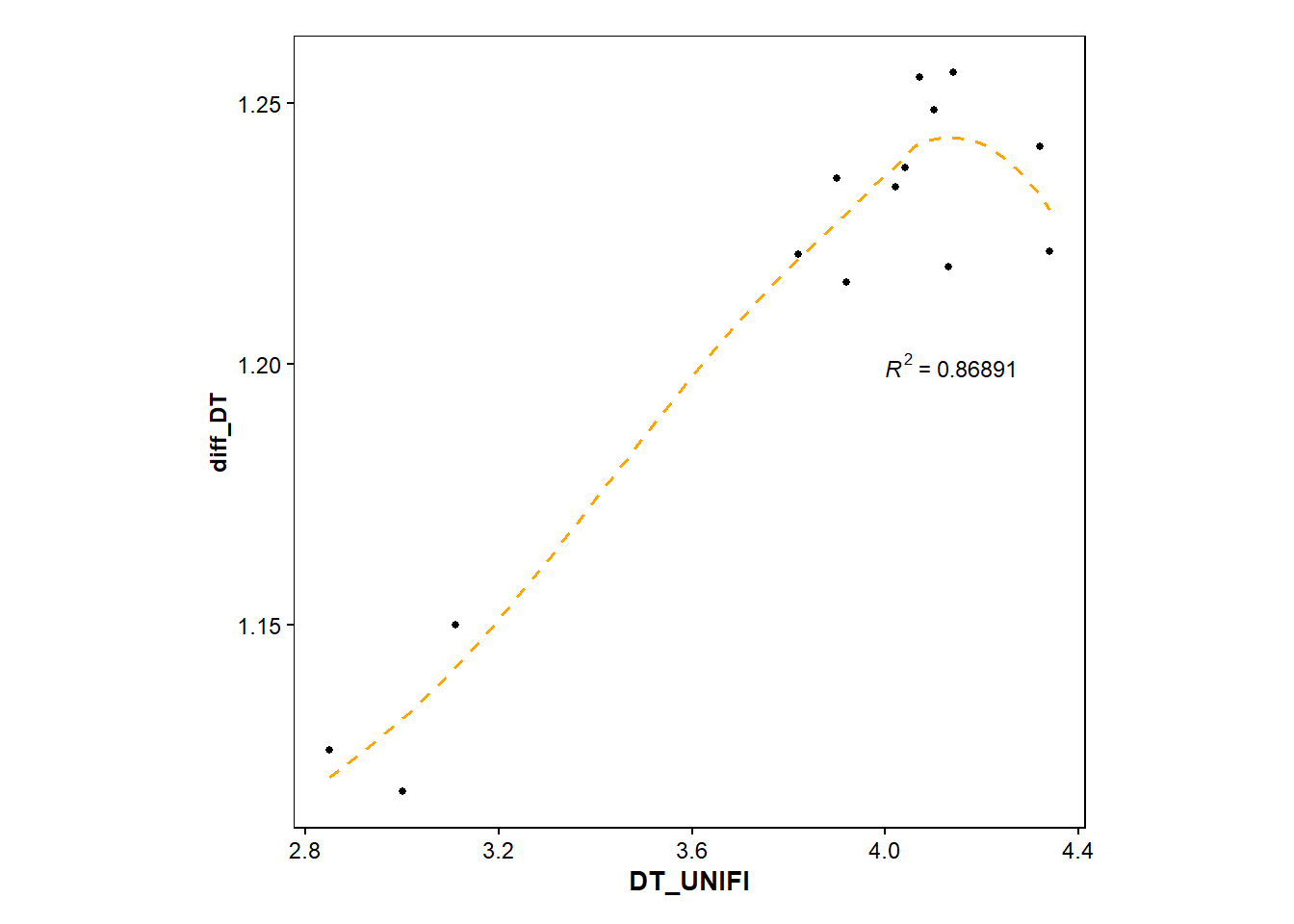
ggarrange(p3, p4,
          labels = c("A", "B"),
          #ncol = 1, nrow = 2,
          widths = 2, heights = 10)
`geom_smooth()` using formula = 'y ~ x'Warning: Removed 3 rows containing non-finite outside the scale range
(`stat_smooth()`).Warning: Removed 3 rows containing non-finite outside the scale range
(`stat_cor()`).Warning: Removed 3 rows containing missing values or values outside the scale range
(`geom_point()`).`geom_smooth()` using formula = 'y ~ x'Warning: Removed 3 rows containing non-finite outside the scale range
(`stat_smooth()`).Warning: Removed 3 rows containing non-finite outside the scale range
(`stat_cor()`).Warning: Removed 3 rows containing missing values or values outside the scale range
(`geom_point()`).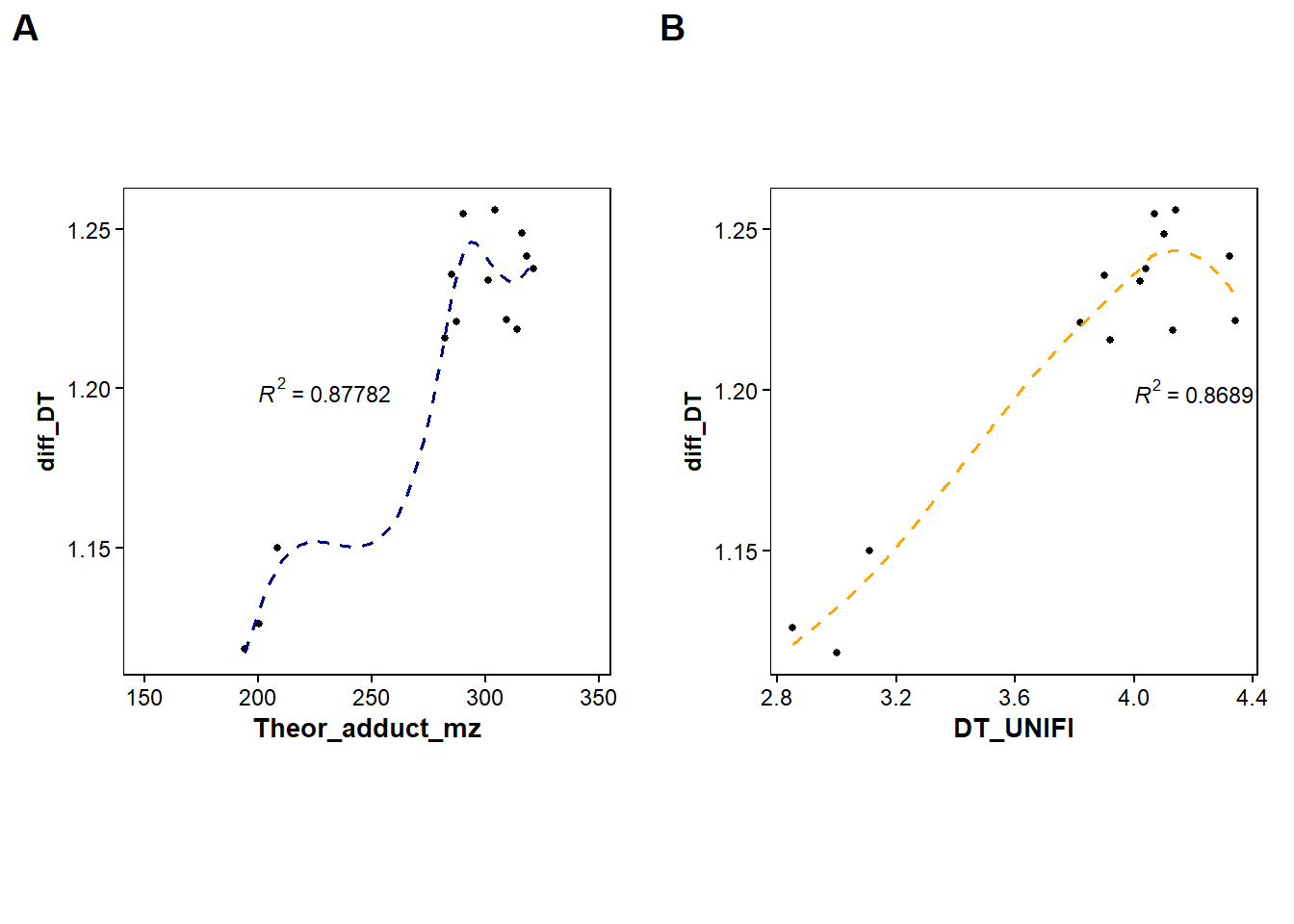
#Import and find the IS compounds in the processed durg mixture data
target_IS <- read_excel("C:/Users/vicer06/OneDrive - Linköpings universitet/Documents/01_Projects/01_VION_HRMS_MSConvert_Processing_2024/Illicit_Drugs_Files/illicit drugs CS-IS_data.xlsx", na = "NA") |>
  filter(Class=="IS") |>
  select(-`Monoisomass`, -`Adduct_ion`,  -`Vion_observed_mz`, -`Agilent_observed_mz`, -`Agilent_RT`)


found_IS <- target_IS |> inner_join(data_drugmix, join_by(overlaps("Theor_adduct_mz","Theor_adduct_mz","mz_range:min", "mz_range:max"))) |>
  select(1:11, mz, height, everything()) |>  #reorder columns
  mutate(Mass_error_ppm = mass_error(Theor_adduct_mz, mz), .after = "mz")

filtered_found_IS <- found_IS |>  slice_min(by=Compound, abs(Mass_error_ppm)) #only keeps the rows with the smallest absolut mass error for each compound


#normalise the heights for the new and old with the IS corresponding IS
normalisation_IS <- inner_join(x=filtered_found_drugs, y=filtered_found_IS, join_by(x$Formula == y$Formula)) |>
  mutate(normalised_height_NEW = `datafile:Drugdtd-200ppb-newsetting_1_A,2_1.mzML:height.x`/`datafile:Drugdtd-200ppb-newsetting_1_A,2_1.mzML:height.y`, .after="height.x") |>
  mutate(normalised_height_OLD = `datafile:Drugstd-200ppb_1_A,3_1.mzML:height.x`/`datafile:Drugstd-200ppb_1_A,3_1.mzML:height.y`, .after="height.x") |>
  mutate(RT_diff = rt.x-rt.y, .after="rt.x") |>
  mutate(mz_error_diff = Mass_error_ppm.x-Mass_error_ppm.y, .after="mz.x") |>
  mutate(DT_diff = ion_mobility.x-ion_mobility.y, .after="ion_mobility.x")

######################################################################
normalisation_IS$plot <- NA #empy column to put plot in
plot_object <- ggplot(data = normalisation_IS, aes(x=normalised_height_OLD, y=normalised_height_NEW))+geom_point(colour="darkgreen")+theme_minimal()+theme(legend.position="none")  #create plot object to put in empty colum in the table

#library(gt) #package for makeing tables + library(gtExtras) # plot in table

#creates a table of selected column from normalisation_IS data
 gt_tab <- normalisation_IS |> select(Compound.x, Formula, RT_diff, DT_diff, mz_error_diff, normalised_height_OLD, normalised_height_NEW,plot) |>
    gt() |>
   tab_options(table.font.color="black")|>
    tab_header(
      title=md("**Drug mixture - 200 ppb**"), #**to make bold
      subtitle =md("For **new** and **old** MS settings analytes with corresponding *Internal Standard*") #* to make italic
      ) |>
    fmt_number(columns = c(RT_diff, DT_diff, mz_error_diff,normalised_height_OLD, normalised_height_NEW), decimals=3) |>  #to formate numbers, can select specific columns to display certain nr. of deicmals for example.
    tab_footnote(
    footnote = "Isomeric compounds. They have been matched to the same feature, hence, the reason for the identical values.",
    locations = cells_body(columns = Compound.x, rows = 1:2)
  ) |>
    tab_footnote(
    footnote = md("The large mass error difference between *analyte* and *IS* is due to a larger mass error for the corresponding IS (10.9 compared to analyte -0.101)"),
    locations = cells_body(
      columns = mz_error_diff,
      rows = mz_error_diff == min((mz_error_diff))
    )
  ) |>
    tab_row_group(
    label = md("*Methamphetamine-d9*"), #or can use gt(groupname_col="Compound.y") to add groupnames for all analytes
    rows = 1:2
  ) |>
    tab_spanner(
    label = "Analyte Information",
    columns = c(Compound.x, Formula)
  ) |>
    tab_spanner(
    label = md("Normalisation as <br> *analyte_height/IS_height*"),
    columns = c(normalised_height_OLD, normalised_height_NEW)
  )|>
    tab_spanner(
    label = md("Differences as <br> *Analyte* - *IS*"),
    columns = c(RT_diff, DT_diff, mz_error_diff)
  ) |>
    cols_label(
    Compound.x = html("Analyte Name"),
    Formula = html("Molecular formula"),
    RT_diff = html("Retention Time ,<br>min"),
    DT_diff = html("Drift Time ,<br>ms"),
    mz_error_diff = html("Mass Error,<br>ppm"),
    normalised_height_OLD = html("OLD"),
    normalised_height_NEW = html("NEW"),
  ) |>
   tab_style(
    style = list(
      cell_fill(color = "lightcyan"),
      cell_text(weight = "bold")
      ),
    locations = cells_body(
      columns = normalised_height_OLD
    )
  ) |>
     tab_style(
    style = list(
      cell_fill(color = "#F9E3D6"),
      cell_text(weight = "bold")
      ),
    locations = cells_body(
      columns = normalised_height_NEW
    )
  ) |>
    tab_style(
    style = list(
      cell_text(color="red")
      ),
    locations = cells_body(
      columns = mz_error_diff,
      rows = mz_error_diff ==min((mz_error_diff))
    )
  )|>
   text_transform(
     locations = cells_body(columns = plot),
     fn = function(x) {
       plot_object |>
         ggplot_image((height=px(200)))
     }
   )
gt_tab| Drug mixture - 200 ppb | |||||||
| For new and old MS settings analytes with corresponding Internal Standard | |||||||
| Analyte Information |
Differences as Analyte - IS |
Normalisation as analyte_height/IS_height |
plot | ||||
|---|---|---|---|---|---|---|---|
| Analyte Name | Molecular formula | Retention Time , min |
Drift Time , ms |
Mass Error, ppm |
OLD | NEW | |
| Methamphetamine-d9 | |||||||
| Phentermine1 | C10H15N | 0.017 | 0.000 | 1.115 | 0.642 | 0.365 |  |
| Methamphetamine1 | C10H15N | 0.017 | 0.000 | 1.115 | 0.642 | 0.365 | |
| MDMA | C11H15NO2 | 0.015 | −0.024 | −1.235 | 1.716 | 1.290 | |
| MDEA | C12H17NO2 | 0.012 | −0.024 | −0.635 | 1.663 | 2.001 | |
| Benzoylecgonine | C16H19NO4 | 0.000 | 0.000 | −0.404 | 2.419 | 2.320 | |
| THC-COOH | C21H28O4 | −0.002 | −0.095 | 2 −11.002 | 3.269 | 2.502 | |
| 1 Isomeric compounds. They have been matched to the same feature, hence, the reason for the identical values. | |||||||
| 2 The large mass error difference between analyte and IS is due to a larger mass error for the corresponding IS (10.9 compared to analyte -0.101) | |||||||
#gt_tab |> gtsave(filename = "tab_1.html") #saves the table in HTML format
#gt_tab |> gtsave(filename = "tab_1.tex") #saves the table in LaTEX format
#gt_tab |> gtsave(filename = "tab_1.docx") #saves the table in WORD format


agg_iris = normalisation_IS  |>
    group_by(Compound.x)  |>
    reframe(
        normalised_height= list(normalised_height_OLD, normalised_height_NEW),
    )

agg_iris |> gt() |> gt_plt_sparkline(column = normalised_height)
`geom_line()`: Each group consists of only one observation.
ℹ Do you need to adjust the group aesthetic?
`geom_line()`: Each group consists of only one observation.
ℹ Do you need to adjust the group aesthetic?
`geom_line()`: Each group consists of only one observation.
ℹ Do you need to adjust the group aesthetic?
`geom_line()`: Each group consists of only one observation.
ℹ Do you need to adjust the group aesthetic?
`geom_line()`: Each group consists of only one observation.
ℹ Do you need to adjust the group aesthetic?
`geom_line()`: Each group consists of only one observation.
ℹ Do you need to adjust the group aesthetic?
`geom_line()`: Each group consists of only one observation.
ℹ Do you need to adjust the group aesthetic?
`geom_line()`: Each group consists of only one observation.
ℹ Do you need to adjust the group aesthetic?
`geom_line()`: Each group consists of only one observation.
ℹ Do you need to adjust the group aesthetic?
`geom_line()`: Each group consists of only one observation.
ℹ Do you need to adjust the group aesthetic?
`geom_line()`: Each group consists of only one observation.
ℹ Do you need to adjust the group aesthetic?
`geom_line()`: Each group consists of only one observation.
ℹ Do you need to adjust the group aesthetic?| Compound.x | normalised_height |
|---|---|
| Benzoylecgonine | |
| Benzoylecgonine | |
| MDEA | |
| MDEA | |
| MDMA | |
| MDMA | |
| Methamphetamine | |
| Methamphetamine | |
| Phentermine | |
| Phentermine | |
| THC-COOH | |
| THC-COOH |
3.3 Drug mix 2024-03-20
The drug mixture has been measured as above, but has been measured with different settings such as LC-gradient, desolvation temperature, etc.
#Import the data and calculate the mass error depending on the the adduct the compounds is found as
drugmix <- read_excel("C:/Users/vicer06/OneDrive - Linköpings universitet/Documents/01_Projects/01_VION_HRMS_MSConvert_Processing_2024/Illicit_Drugs_Files/illicit drugs CS-IS_data - MassErrors_Calculations.xlsx",
    sheet = "Drugmix_240320_21 (2)")
drugmix <- drugmix |>
  mutate(Mass_acc=case_when(`mode...14` == "[M+H]+" ~ mass_error(Theor_adduct_mz, `m/z...9`),
                            `mode...14` == "[M+Na]+" ~ mass_error(`Theor. [M+Na]+`, `m/z...9`),
                            `mode...14` == "[M+NH4]+" ~ mass_error(`Theor. [M+NH4]+`, `m/z...9`)), .after=`mode...14`) |>
  mutate(Mass_acc2=case_when(`mode...21` == "[M+H]+" ~ mass_error(Theor_adduct_mz, `m/z...16`),
                            `mode...21` == "[M+Na]+" ~ mass_error(`Theor. [M+Na]+`, `m/z...16`),
                            `mode...21` == "[M+NH4]+" ~ mass_error(`Theor. [M+NH4]+`, `m/z...16`)), .after=`mode...21`) |>
  mutate(Mass_acc3=case_when(`mode...28` == "[M+H]+" ~ mass_error(Theor_adduct_mz, `m/z...23`),
                            `mode...28` == "[M+Na]+" ~ mass_error(`Theor. [M+Na]+`, `m/z...23`),
                            `mode...28` == "[M+NH4]+" ~ mass_error(`Theor. [M+NH4]+`, `m/z...23`)), .after=`mode...28`) |>
  mutate(Mass_acc4=case_when(`mode...35` == "[M+H]+" ~ mass_error(Theor_adduct_mz, `m/z...30`),
                            `mode...35` == "[M+Na]+" ~ mass_error(`Theor. [M+Na]+`, `m/z...30`),
                            `mode...35` == "[M+NH4]+" ~ mass_error(`Theor. [M+NH4]+`, `m/z...30`)), .after=`mode...35`) |>
  mutate(Mass_acc5=case_when(`mode...42` == "[M+H]+" ~ mass_error(Theor_adduct_mz, `m/z...37`),
                            `mode...42` == "[M+Na]+" ~ mass_error(`Theor. [M+Na]+`, `m/z...37`),
                            `mode...42` == "[M+NH4]+" ~ mass_error(`Theor. [M+NH4]+`, `m/z...37`)), .after=`mode...42`)

##DID NOT WORK AS INTENDEN DUE TO THE FORMAT OF THE EXCEL SHEET##########
drugmix |>
  pivot_longer(cols = c(`detector count...13`, `detector count...20`, `detector count...27`, `detector count...34`,`detector count...41`),
                            names_to = "detectorcoun_comb",
                            values_to = "Intensities")
# A tibble: 105 × 53
Compound Class Formula Monoisomass Theor_adduct_mz `Theor. [M+Na]+`
<chr> <chr> <chr> <dbl> <dbl> <dbl>
1 3,4-methylenediox… Anal… C10H13… 179. 180. 202.
2 3,4-methylenediox… Anal… C10H13… 179. 180. 202.
3 3,4-methylenediox… Anal… C10H13… 179. 180. 202.
4 3,4-methylenediox… Anal… C10H13… 179. 180. 202.
5 3,4-methylenediox… Anal… C10H13… 179. 180. 202.
6 6-acetylmorphine Anal… C19H21… 327. 328. 350.
7 6-acetylmorphine Anal… C19H21… 327. 328. 350.
8 6-acetylmorphine Anal… C19H21… 327. 328. 350.
9 6-acetylmorphine Anal… C19H21… 327. 328. 350.
10 6-acetylmorphine Anal… C19H21… 327. 328. 350.
# ℹ 95 more rows
# ℹ 47 more variables: `Theor. [M+NH4]+` <dbl>,
# `UNIFI - HDMSe-destemp450_240320` <lgl>, `m/z...9` <dbl>,
# `RT [min]...10` <dbl>, DT...11 <dbl>, CCS...12 <dbl>, mode...14 <chr>,
# Mass_acc <dbl>, `UNIFI - HDMSe-gradientchange_240320` <lgl>,
# `m/z...16` <dbl>, `RT [min]...17` <dbl>, DT...18 <dbl>, CCS...19 <dbl>,
# mode...21 <chr>, Mass_acc2 <dbl>, …#################################
#plot the intensities of the compounds for each type of measurement
f1 <- ggplot(drugmix, aes(x=Theor_adduct_mz, y=`detector count...13`))+
geom_point()+
geom_point(aes(x=Theor_adduct_mz, y=`detector count...20`), color="red")+
geom_point(aes(x=Theor_adduct_mz, y=`detector count...27`), color="green")+
geom_point(aes(x=Theor_adduct_mz, y=`detector count...34`), color="blue")+
geom_point(aes(x=Theor_adduct_mz, y=`detector count...41`), color="orange")+
labs( y = "Detector Count", x=expression(paste("Theoretical ",italic("m/z"), " values"))) +
theme_minimal()+
theme(
panel.background = element_rect(fill = "white"), # Set white background
panel.grid.major = element_blank(), # Remove grid lines
panel.grid.minor = element_blank(), # Remove grid lines
axis.text = element_text(size = 9), # Increase font size of axis text
axis.title.y = element_text(size = 9,face = "bold"), # Make y-axis label bold and italic
axis.text.y = element_text(color = "black", size = 9), # Make x-axis text bold
axis.title.x = element_text(size = 10,face = "bold"),
axis.text.x = element_text(color = "black", size = 9), # Make x-axis text bold
axis.ticks.x = element_line(color = "black"), # Add ticks to x-axis in black color
axis.ticks.y = element_line(color = "black"), # Add ticks to y-axis in black color
plot.margin = margin(0.5, 0.5, 0.4, 0.5, "cm"), # Set plot margins
legend.text=element_text(size=9),
legend.background = element_rect(fill="white",
size=0.5, linetype="solid",
colour ="black"),
legend.title = element_blank(),
)
#plot the mass error for the compounds for each measurement
f2 <-ggplot(drugmix, aes(x=Compound, y=Mass_acc))+
geom_point()+
geom_point(aes(y=Mass_acc2), color="red")+
geom_point(aes(y=Mass_acc3), color="green")+
geom_point(aes(y=Mass_acc4), color="blue")+
geom_point(aes(y=Mass_acc5), color="orange")+
labs( y = "Mass Accuracy [ppm]", x=" ") +
theme_minimal()+
theme(
panel.background = element_rect(fill = "white"), # Set white background
panel.grid.major = element_blank(), # Remove grid lines
panel.grid.minor = element_blank(), # Remove grid lines
axis.text = element_text(size = 9), # Increase font size of axis text
axis.title.y = element_text(size = 9,face = "bold"), # Make y-axis label bold and italic
axis.text.y = element_text(color = "black", size = 9), # Make x-axis text bold
axis.title.x = element_text(size = 10,face = "bold"),
axis.text.x = element_text(color = "black", size = 9, angle = 45, hjust = 1), # Make x-axis text bold
axis.ticks.x = element_line(color = "black", ), # Add ticks to x-axis in black color
axis.ticks.y = element_line(color = "black"), # Add ticks to y-axis in black color
plot.margin = margin(0.5, 0.5, 0.4, 0.5, "cm"), # Set plot margins
legend.text=element_text(size=9),
legend.background = element_rect(fill="white",
size=0.5, linetype="solid",
colour ="black"),
legend.title = element_blank(),
)
#plot the CCS for the compounds for each measurement
f3 <- ggplot(drugmix, aes(x=Theor_adduct_mz, y=`CCS...12`))+
geom_point()+
geom_point(aes(x=Theor_adduct_mz, y=`CCS...19`), color="red")+
geom_point(aes(x=Theor_adduct_mz, y=`CCS...26`), color="green")+
geom_point(aes(x=Theor_adduct_mz, y=`CCS...33`), color="blue")+
geom_point(aes(x=Theor_adduct_mz, y=`CCS...40`), color="orange")+
labs( y = "Drift Time", x=expression(paste("Theoretical ",italic("m/z"), " values"))) +
theme_minimal()+
theme(
panel.background = element_rect(fill = "white"), # Set white background
panel.grid.major = element_blank(), # Remove grid lines
panel.grid.minor = element_blank(), # Remove grid lines
axis.text = element_text(size = 9), # Increase font size of axis text
axis.title.y = element_text(size = 9,face = "bold"), # Make y-axis label bold and italic
axis.text.y = element_text(color = "black", size = 9), # Make x-axis text bold
axis.title.x = element_text(size = 10,face = "bold"),
axis.text.x = element_text(color = "black", size = 9), # Make x-axis text bold
axis.ticks.x = element_line(color = "black"), # Add ticks to x-axis in black color
axis.ticks.y = element_line(color = "black"), # Add ticks to y-axis in black color
plot.margin = margin(0.5, 0.5, 0.4, 0.5, "cm"), # Set plot margins
legend.text=element_text(size=9),
legend.background = element_rect(fill="white",
size=0.5, linetype="solid",
colour ="black"),
legend.title = element_blank(),
)
ggarrange(f2, f1, f3,
labels = c("A", "B", "C"),
ncol=3)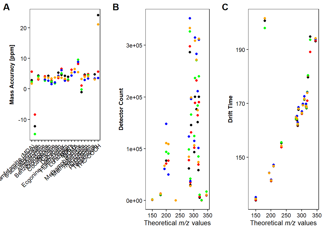
f3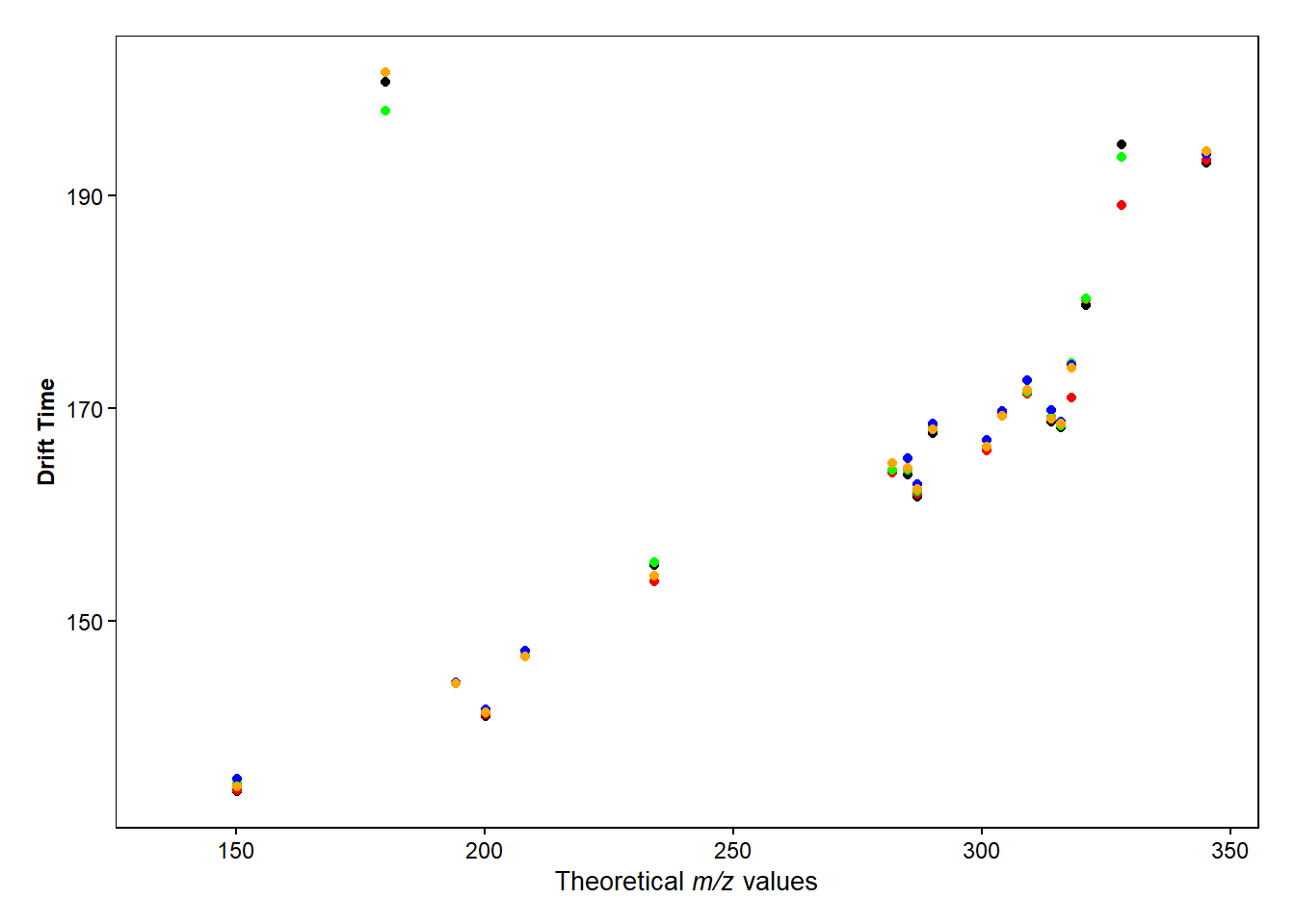
TidyMass
#source("https://www.tidymass.org/tidymass-packages/install_tidymass.txt")
#install_tidymass(from = "tidymass.org")
EstimatePrecursorMz
#library(Spectra)
#fls <- system.file("C:/Users/vicer06/OneDrive - Linköpings universitet/Documents/01_Projects/01_VION_HRMS_MSConvert_Processing_2024/Drugmixture_MSconvert_Processing_240321")
#sps_sciex <- Spectra(fls, source = MsBackendMzR())
#sps_sciex