5  Familiarization of Raw Data - IMS-HRMS

https://rformassspectrometry.github.io/book/sec-raw.html

5.0.1 Loading of libraries

if (!requireNamespace("BiocManager", quietly = TRUE))
    install.packages("BiocManager")

BiocManager::install("tidyverse")
BiocManager::install("factoextra")
BiocManager::install("msdata")
BiocManager::install("mzR")
BiocManager::install("rhdf5")
BiocManager::install("rpx")
BiocManager::install("MsCoreUtils")
BiocManager::install("QFeatures")
BiocManager::install("Spectra")
BiocManager::install("ProtGenerics")
BiocManager::install("PSMatch")
BiocManager::install("pheatmap")
BiocManager::install("limma")
BiocManager::install("MSnID")
BiocManager::install("RforMassSpectrometry/SpectraVis")

library(mzR)
library(Spectra)
library(tidyverse)
library(viridis)
library(patchwork)

#Combined IMS
#mz_ims2 <- "C:\\Users\\vicer06\\OneDrive - Linköpings universitet\\Documents\\01_Projects\\01_VION_HRMS_MSConvert_Processing_2024\\Test_Spectra_Function_R\\Drugstd-200ppb_1_A,3_1-Combined.mzML"
#sp_ims2 <- Spectra(mz_ims2)

#IMS-HRMS data
mz_ims <- "C:\\Users\\vicer06\\OneDrive - Linköpings universitet\\Documents\\01_Projects\\01_VION_HRMS_MSConvert_Processing_2024\\Test_Spectra_Function_R\\Drugstd-200ppb_1_A,3_1.mzML"

sp_ims <- Spectra(mz_ims)
# glimpse(sp_ims) #view structure of file
# length(sp_ims) #number of scans
# 
# spectraVariables(sp_ims) #Extract metadata varaibles
# 
# sp_ims[["peaksCount"]] #Use metadata variables to extract them
# sp_ims[["ionMobilityDriftTime"]]
# sp_ims[["rtime"]]
# sp_ims[["msLevel"]]
# #or can use
# rtime(sp_ims)
# scanIndex(sp_ims)
# msLevel(sp_ims)
# 
# spectraData(sp_ims) #Extract all metadata
# 
# raw_data_ims <- peaksData(sp_ims) #Extract list with all raw data
# 
# ####for help ?Spectra####
# 
# filterAcquisitionNum(sp_ims, n=2000:2001) #filter for scan 2000-2001 in sp_ims
# 
# filterIntensity(
#     sp_ims,
#     intensity = c(10000, Inf)#,
#     #msLevel. = uniqueMsLevels(sp_ims)
# ) #filter for intensities, removes peaks below 10 000 in intensity
# 
# filterMsLevel(sp_ims, msLevel. = 1) #filter for MS levels, here for MS1
# 
# filterRt(sp_ims, rt = 1:2, uniqueMsLevels(sp_ims)) #filter for Retention time, here between 1 and 2

5.0.2 Plot Mass Spectrum

#plotSpectra can bu used to plot the Mass spectrum of a scan. In the raw data (Spectrum("xxx.mzML")), one can find ""peaksVariables" containing "mz" and "intensity", which tells what to use for the plot??

# #Plot Spectra of a scan and displays the m/z with a smaller font size
# plotSpectra(sp_ims[1800], labels = function(z) format(unlist(mz(z))), labelCex=0.5) #MS1
# plotSpectra(sp_ims[1801], labels = function(z) format(unlist(mz(z))), labelCex=0.5) #MS2
# 
# plotSpectra(filterAcquisitionNum(sp_ims, n=1800:1801)) #Both MS1 and MS2 at same time
# 
# 
# plotSpectra(filterMsLevel(sp_ims, msLevel. = 1)[1800], labels = function(z) format(unlist(mz(z))))
# plotSpectra(filterMsLevel(sp_ims, msLevel. = 2)[1800], labels = function(z) format(unlist(mz(z))))
# 
# plotSpectraOverlay(filterMsLevel(sp_ims, msLevel. = 1)[1:200]) #overlay the spectran for scan nr1 to nr200 for MS1

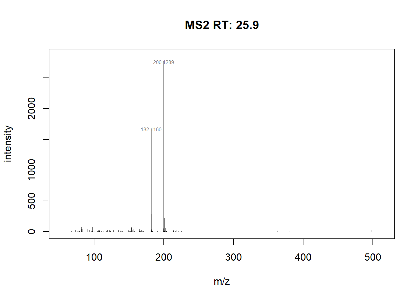
#plot scan 24655, and labels the peaks above 500 intensity and smaller font size
plotSpectra(sp_ims[24655], labelCex=0.5,
            labels = function(z) {
        lbls <- format(mz(z)[[1L]], digits=6)
        lbls[intensity(z)[[1L]] <= 500] <- ""
        lbls
    })

5.0.3 Constructing a TIC of the data

################### TIC MS1 ##############################
# sp_ims_ms1 <- filterMsLevel(sp_ims, msLevel. = 1) #filter for MS levels, here for MS1
# 
# mz_ms1 <- mz(sp_ims_ms1)
# rtime_ms1 <- rtime(sp_ims_ms1)
# intensity_ms1 <- intensity(sp_ims_ms1)
# scanindex_ms1 <- scanIndex(sp_ims_ms1)

#### Sum intensities for each scan ####

# # Initialize an empty vector to store the sum of intensities
# sum_intensity_ms1 <- numeric(length(scanindex_ms1))
# # Iterate over each scan time
# for (i in seq_along(scanindex_ms1)) {
#   # Sum the intensity values for the current scan time
#   sum_intensity_ms1[i] <- sum(intensity_ms1[[i]])
# }
# 
# ## ionCount(sp_ims) sums the intensities for each scan
# 
# 
# #Plot the summed intensities against the retention times
# with(spectraData(sp_ims_ms1),
#      plot(rtime_ms1, sum_intensity_ms1, type="l"))
# abline(v = rtime(sp_ims_ms1)[24455], col = "red")


#### Sum intensities for each RT ####

# unique_rt_ms1 <- unique(rtime_ms1)
# # Initialize an empty vector to store the sum of intensities
# sum2_intensity_ms1 <- numeric(length(unique_rt_ms1))
# # Iterate over each unique scan time
# for (i in seq_along(unique_rt_ms1)) {
#   # Find the index of the current scan time in the original data
#   idx_ms1 <- which(rtime_ms1 == unique_rt_ms1[i])
#   # Sum the intensity values for the scans with the current scan time
#   sum2_intensity_ms1[i] <- sum(unlist(intensity_ms1[idx_ms1]))
# }
# #Plot the summed intensities against the retention times
# with(spectraData(sp_ims_ms1),
#      plot(unique_rt_ms1/60, sum2_intensity_ms1, type="l",
#           xlab="RT", ylab= "Summed Intensities",
#           main = "Sum Intensties MS1",
#           xlim=c(0.3,8.4)))

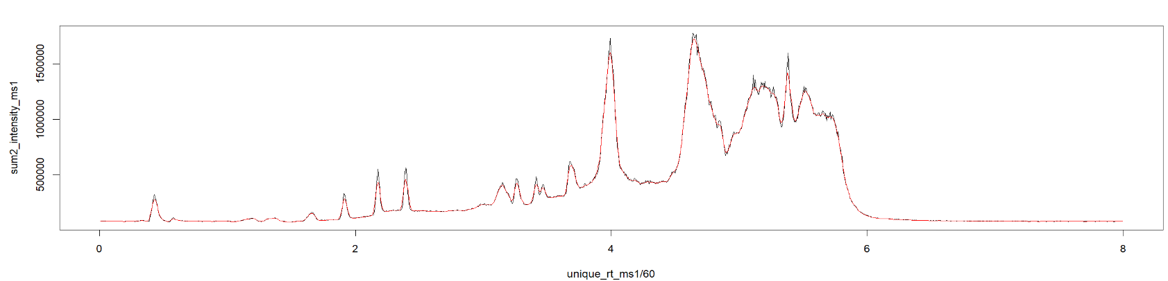
######overlaying of msdial TIC and MS1 TIC
  #  plot(unique_rt_ms1/60, sum2_intensity_ms1, type="l")
  #  lines(msdial$RETENTIONTIME, msdial$INTENSITY, col="red")


############################ TIC all MS #####################################

#Saves m/z, RT, Intensity, and scanIndex as new objects
mz <- mz(sp_ims) #not needed for tic
scanindex <- scanIndex(sp_ims) #not needed for tic
rtime <- rtime(sp_ims)
intensity <- intensity(sp_ims)

unique_rt <- unique(rtime) #Finds the uniques retention times since the same RT exists for multiple scans

# Create an empty vector to store the sum of intensities
sum2_intensity <- numeric(length(unique_rt))

# Iterate over each unique scan time
for (i in seq_along(unique_rt)) {
  # Find the index of the current scan time in the original data
  idx <- which(rtime == unique_rt[i])
  # Sum the intensity values for the scans with the current scan time
  sum2_intensity[i] <- sum(unlist(intensity[idx]))
}
#Plot the retention times against the summed intensities
with(spectraData(sp_ims),
     plot(unique_rt/60, sum2_intensity, type="l",
          xlab="RT [min]", ylab= "Summed Intensities",
          main = "TIC",
          xlim=c(0.3,8.4),
          ylim=c(0,3.0e6)))
abline(v = rtime(sp_ims)[267139]/60, col = "red") #adds red line for scan 267139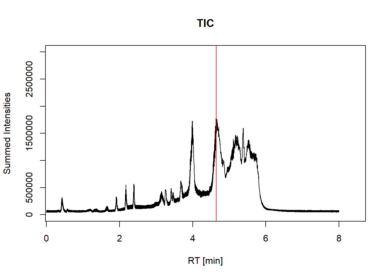

max(sum2_intensity) #find maximum intensity in TIC

[1] 1775374

#plots spectrum for scan 267139
plotSpectra(sp_ims[267139], labelCex=0.6,
            labels = function(z) {
        lbls <- format(mz(z)[[1L]], digits=6)
        lbls[intensity(z)[[1L]] <= 500] <- ""
        lbls
    })

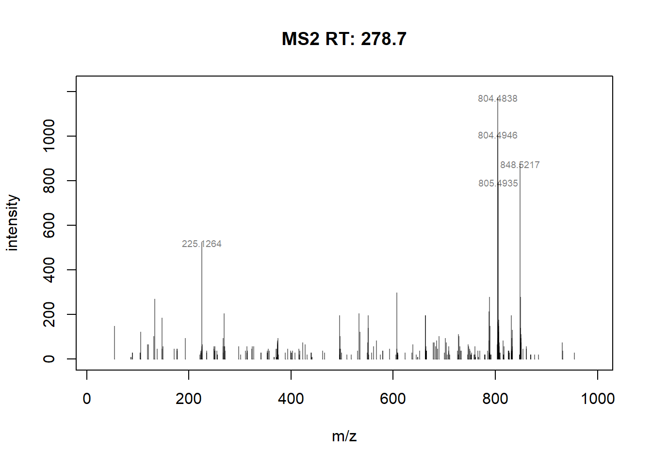
max(intensity[267139]) #find maximum intensity at scan 267139

[1] 1173

Comparion of TIC of drug-mixture (200 ppb, old-settings) with other softwares:

• TIC MS1MS2 - R code (time ⁓ 56 + 46 sec)

  

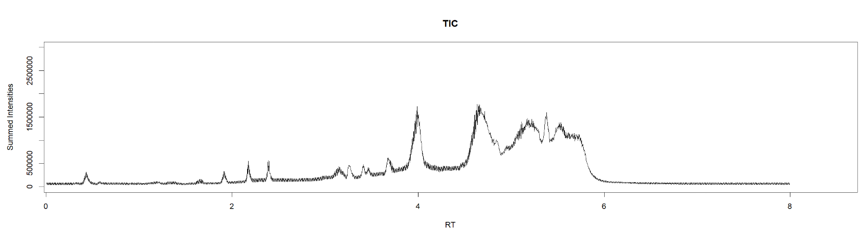
• SeeMS - Higher intensities (time ⁓ 50sec)

  

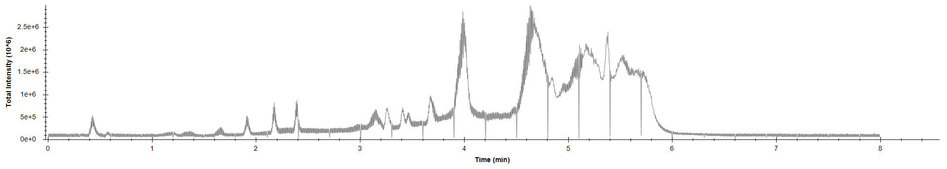
• MS-DIAL (first needs to process the file, then can open TIC, time ⁓ 10 min )

  

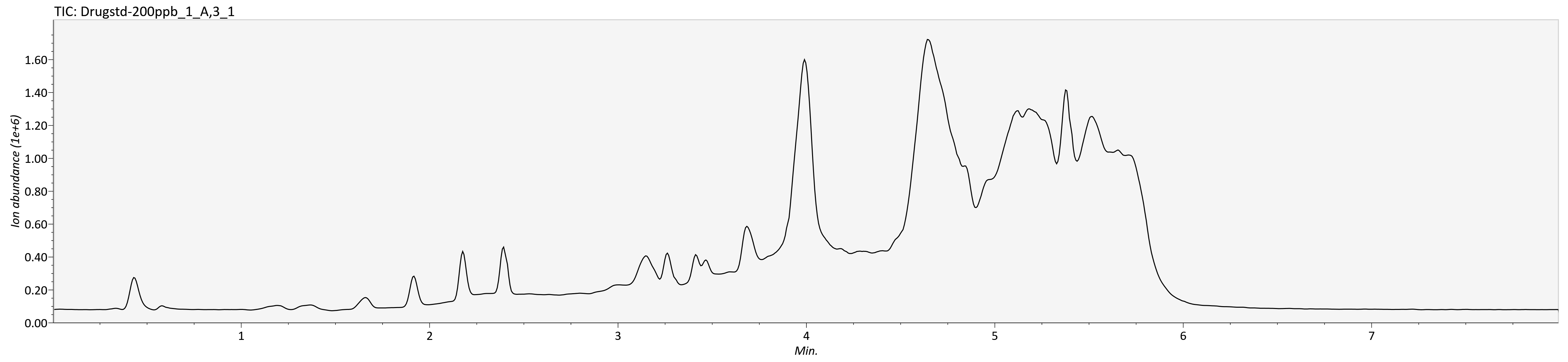
  • Overlaying TIC MS1 (black) and TIC MSDIAL (red)

    

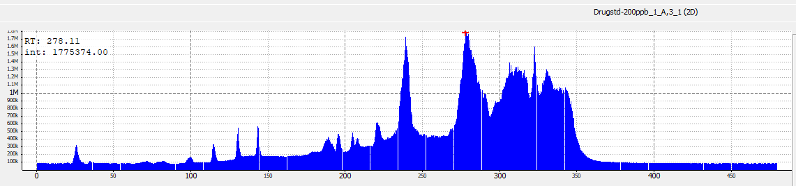
• ToppView (time ⁓ 1.22 min)

  

##Drift time Summed inteisities

intensity <- intensity(sp_ims)
dtime <- sp_ims[["ionMobilityDriftTime"]]

unique_dt <- unique(dtime) #Finds the uniques retention times since the same RT exists for multiple scans

# Create an empty vector to store the sum of intensities
sum3_intensity <- numeric(length(unique_dt))

# Iterate over each unique scan time
for (i in seq_along(unique_dt)) {
  # Find the index of the current scan time in the original data
  idx <- which(dtime == unique_dt[i])
  # Sum the intensity values for the scans with the current scan time
  sum3_intensity[i] <- sum(unlist(intensity[idx]))
}
#Plot the retention times against the summed intensities
with(spectraData(sp_ims),
     plot(unique_dt, sum3_intensity, type="l",
          xlab="DT [ms]", ylab= "Summed Intensities",
          main = "Drift Time Summed Intensities"))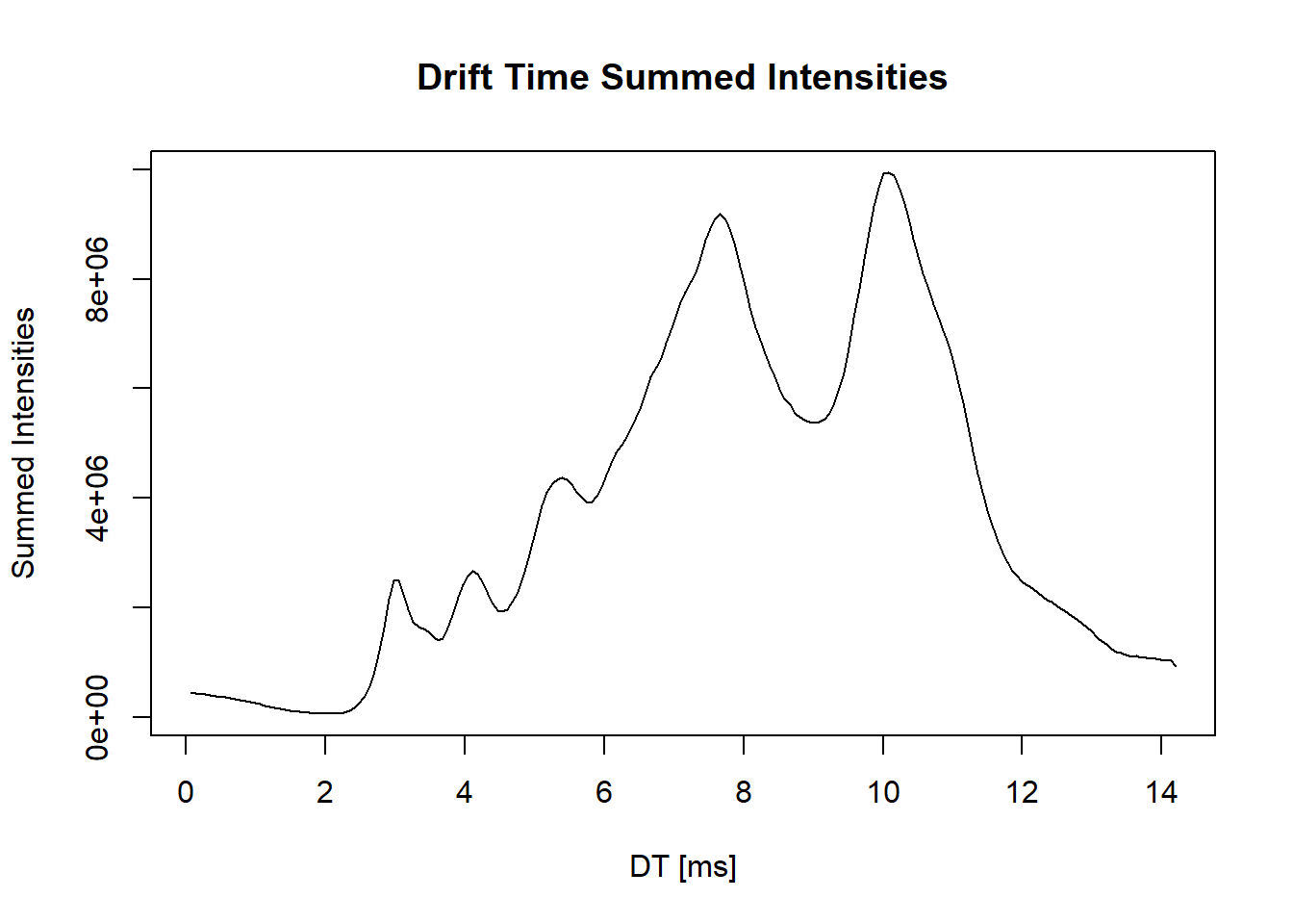

#######################################################################
#PLOT of Retention time vs Drift time and Intensities
test_intensities <- ionCount(sp_ims)
data <- data.frame(dtime,
                   rtime ,
                   test_intensities)
ggplot(data, aes(x=rtime/60, y=dtime))+
  geom_point(aes(color=test_intensities))+
  scale_color_viridis(discrete=FALSE)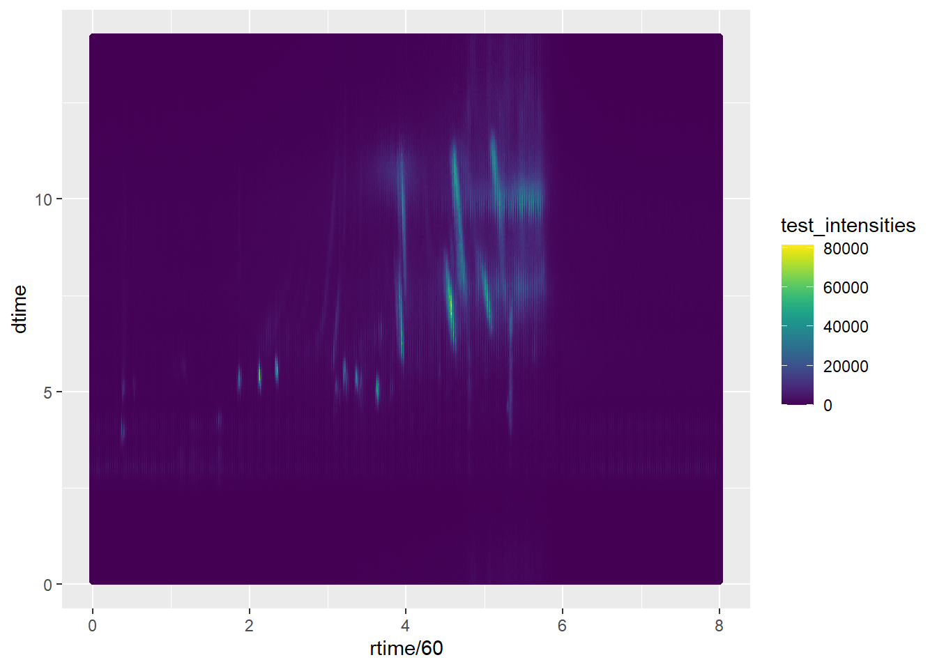

############# To arrange RT VS DT plot with the RT and DT TIC ###########
gg <- ggplot(data, aes(x=rtime/60, y=dtime))+
  geom_point(aes(color=test_intensities))+
  scale_color_viridis(discrete=FALSE)+
  scale_x_continuous(expand=c(0, 0),limits=c(0, max(rtime)/60))+
  scale_y_continuous(expand=c(0, 0), limits=c(0, max(dtime)))+
  labs(y = "Drift Time [ms]", x= "Retention Time [min]")+
  theme_minimal()+
  theme(legend.title = element_blank(),
        legend.position = c(.9,.75),
        legend.text=element_text(size=9),
        legend.background = element_rect(fill="white",
                                         colour ="white"),
        panel.grid.major = element_blank(),
        panel.grid.minor = element_blank(),
        plot.margin = margin(-1, -1, -1, -1, "cm"),
        axis.ticks.x = element_line(color = "black"), 
        axis.ticks.y = element_line(color = "black"),
        panel.border = element_rect(colour = "black", fill=NA, size=.5))

Warning: The `size` argument of `element_rect()` is deprecated as of ggplot2 3.4.0.
ℹ Please use the `linewidth` argument instead.

Warning: A numeric `legend.position` argument in `theme()` was deprecated in ggplot2
3.5.0.
ℹ Please use the `legend.position.inside` argument of `theme()` instead.

#make data fram of TIC to be abel to use ggplot
d1 <- data.frame(unique_rt, sum2_intensity) 
d2 <- data.frame(unique_dt, sum3_intensity)
g1 <- ggplot(d1, aes(x=unique_rt/60, y=sum2_intensity))+
  geom_line()+
  scale_x_continuous(expand=c(0, 0))+
  scale_y_continuous(expand=c(0, 0))+
  theme_minimal()+
  theme(axis.text.x=element_blank(), 
      axis.ticks.x=element_blank(), 
      axis.text.y=element_blank(), 
      axis.ticks.y=element_blank(),
      axis.title.x = element_blank(),
      axis.title.y = element_blank(),
      panel.grid.major = element_blank(),
      panel.grid.minor = element_blank())
g2 <- ggplot(d2, aes(x=unique_dt, y=sum3_intensity))+
  geom_line()+
  scale_x_continuous(expand=c(0, 0))+
  scale_y_continuous(expand=c(0, 0))+
  theme_minimal() +
  theme(axis.text.x=element_blank(), 
      axis.ticks.x=element_blank(), 
      axis.text.y=element_blank(), 
      axis.ticks.y=element_blank(),
      axis.title.x = element_blank(),
      axis.title.y = element_blank(),
      panel.grid.major = element_blank(),
      panel.grid.minor = element_blank())+
  coord_flip()

g3 <- plot_spacer() #blank plot to be used in upper right corner



g1 + g3 + gg + g2 +  #arrange the plots with patchwork-package
  plot_layout(widths = c(5, 1), 
              heights = c(1, 5),
              guides = "collect")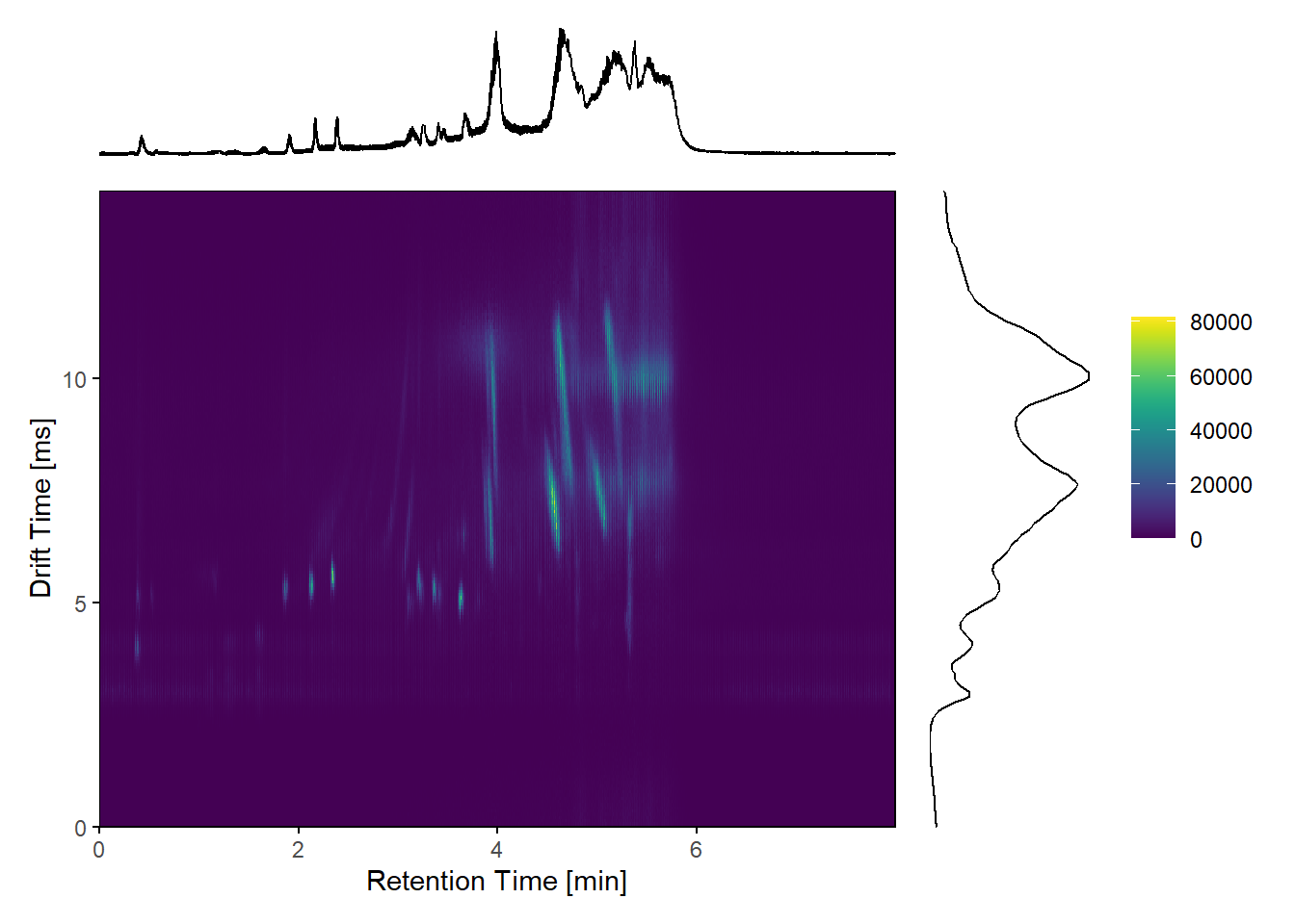

##### RT vs DT MS1 #################
sp_ims_ms1 <- filterMsLevel(sp_ims, msLevel. = 1) #filter for MS levels, here for MS1

dtime_ms1 <- sp_ims_ms1[["ionMobilityDriftTime"]]
rtime_ms1 <- rtime(sp_ims_ms1)
scan_sum_intensities_ms1 <- ionCount(sp_ims_ms1)

dt_rt_int <- data.frame(dtime_ms1,
                   rtime_ms1,
                   scan_sum_intensities_ms1)
ggplot(dt_rt_int, aes(x=rtime_ms1/60, y=dtime_ms1))+
  geom_point(aes(color=scan_sum_intensities_ms1))+
  scale_color_viridis(discrete=FALSE)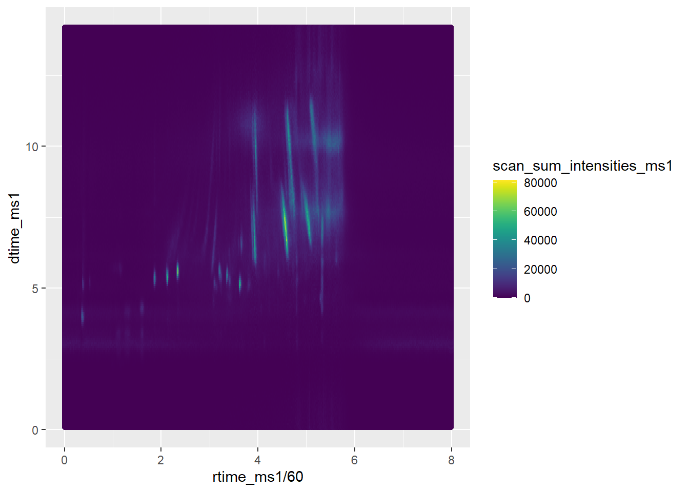

#################### not working ################################################
# mz_ms1 <- mz(sp_ims_ms1)
# intensity_ms1 <- intensity(sp_ims_ms1)
# 
# mz_ms1_unlist <- unlist(mz_ms1)
# int_ms1_unlist <- unlist(intensity_ms1)
# dt_rep_ms1 <- rep(unlist(dtime_ms1), lengths(mz_ms1))
# 
# data2 <- data.frame(dt_rep_ms1,
#                     mz_ms1_unlist,
#                     int_ms1_unlist)
# ggplot(data2, aes(x=mz_ms1_unlist, y=dt_rep_ms1))+
#   geom_point(aes(color=int_ms1_unlist))+
#   scale_color_viridis(discrete=FALSE)
# 
# ## Attempting to make plot of mz vs dt with intensities
# test_intens2 <- unlist(intensity)
# test_mz2 <- unlist(mz)
# 
# dt_rep <- rep(unlist(dtime), lengths(mz))
# 
# data2 <- data.frame(dt_rep,
#                     test_mz2,
#                     test_intens2)
# ggplot(data2, aes(x=test_mz2, y=dt_rep))+
#   geom_point(aes(color=test_intens2))+
#   scale_color_viridis(discrete=FALSE)
# 
# 
# test_mz2
# dtime

5.0.4 XIC of the data

####

# 
# # Plot using ggplot2
# ggplot(data, aes(x = dtime, y = rtime, color = intensity)) +
#   geom_point() +
#   scale_color_gradient(low = "blue", high = "red", na.value = "black") +
#   labs(x = "DTime", y = "RTime", color = "Intensity") +
#   theme_minimal()
# 
# 
# 
# test <- filterMzRange(sp_ims, c(200.128, 200.129))
# 
# test_rt <- rtime(test)
# 
# test <- filterMzValues(sp_ims, c(200.128, 200.129))
# test <- combinePeaks(sp_ims, mz = c(200.12, 200.13))
# 
# test <- filterMzValues(sp_ims, mz = c(103, 104), tolerance = 0.3)
# 
# chromatogram(sp_ims, mz = 200.1)
# 
# 
# 
# test_rt <- rtime(test)
# test_intensity <- intensity(test)
# 
# # Plot the extracted ion chromatogram (XIC)
# with(spectraData(test),
#      plot(test_rt, test_intensity, type = "l")
# )
# 
# mz(test)
# 
# 
# test <- containsMz(
# sp_ims,
# mz = 200.128,
# tolerance = 0.2,
# ppm = 10,
# which = c("any", "all"),
# BPPARAM = bpparam()
# )
# 
# plotSpectra(test)
# 
# peaksData(sp_ims)
# 
# plotSpectra(filterMzValues(sp_ims, c(200.128, 200.129)))
# 
# 
# plotSpectra(sp_ims, xlim = c(521.2, 522.5))

5.0.5 Import more than one file at a time

#import data from folder "Test_Spectra_Function_R" that contains the pattern "Drugstd-200ppb_1_A,3_1", hence data with IMS and combined IMS-dimension are importet
#takes some time to run these
#fls <- dir(path = "C:\\Users\\vicer06\\OneDrive - Linköpings universitet\\Documents\\01_Projects\\01_VION_HRMS_MSConvert_Processing_2024\\Test_Spectra_Function_R", pattern="Drugstd-200ppb_1_A,3_1", full.names = TRUE)
#fls2 <- Spectra(fls)
#table(dataOrigin(fls2)) #show which files been imported

#imports all mzML files in the folder
#fls <- dir(path = "C:\\Users\\vicer06\\OneDrive - Linköpings universitet\\Documents\\01_Projects\\01_VION_HRMS_MSConvert_Processing_2024\\Test_Spectra_Function_R", full.names = TRUE)
#fls2 <- Spectra(fls)
#table(dataOrigin(fls2))

#Backend
#MsBackenedMzR: default, relies on MzR package to read MS data
#MsBackenedMemry: full MS data stored within object (in-memory) to guarantee high performance but on the other hand has higher memory footprint if many mass peaks in specrum
#setBackend(fls2, MsBackendMemory())

---